Review of Multi-scale and Multi-physical Simulation Technologies for Shale and Tight Gas Reservoirs

Article Menu

/ajax/scifeed/subscribe

Open Access Article

Numerical Investigation for Iii-Dimensional Multiscale Fracture Networks Based on a Coupled Hybrid Model

^one

College of Petroleum Engineering, Prc University of Petroleum (Beijing), Beijing 102249, Mainland china

²

Petroleum Engineering School, Southwest Petroleum University, Chengdu 610500, China

ⁱⁱⁱ

Country Primal Laboratory of Petroleum Resources and Prospecting, Communist china University of Petroleum (Beijing), Beijing 102249, Prc

^*

Authors to whom correspondence should be addressed.

Academic Editor: Pål Østebø Andersen

Received: 13 Baronial 2021 / Revised: 22 September 2021 / Accepted: 27 September 2021 / Published: 5 October 2021

Abstract

The mismatching between the multi-scale characteristic of complex fracture networks (CFNs) in unconventional reservoirs and their current numerical approaches is a conspicuous problem to be solved. In this paper, the CFNs are divided into hydraulic macro-fractures, induced fractures, and natural micro-fractures according to their mode of origin. A hybrid model coupling various numerical approaches is proposed to match the iii-dimensional multi-scale fracture networks. The macro-fractures with high-conductivity and wide-aperture are explicitly characterized by a mimetic Green chemical element method-based hierarchical fracture model. The induced fractures and natural micro-fractures that have features of depression-conductivity and small-openings are upscaled to the dual-medium grid and enhanced matrix grid through the equivalent continuum-medium method, respectively. Afterward, some benchmark cases are implemented to confirm the loftier-precision and high-robustness of the proposed hybrid model that indeed accomplishes accurate modeling of fluid flow in multi-scale CFNs by comparing with commercial software tNavigator^®. Furthermore, an integrated workflow of simulation modeling for multiscale CFNs combined with a field instance in Sichuan from People's republic of china is used to analyzing the production data of fractured horizontal wells in shale gas reservoirs. Compared with the field production data from this typical well, it can be proved that the hybrid model has potent reliability and practicability.

one. Introduction

Shale has the characteristics of tight matrix with ultra-low permeability. At nowadays, with the progress of hydraulic fracturing and horizontal well technology, shale gas production has been effectively improved [ane,ii]. Natural fractures developed in multiple tectonic stages, artificial hydraulic fractures reacted by improvement measures, and new connected induced fractures during hydraulic fracturing, combine to plant a multiscale complex fractures system in the shale reservoir. The high-electrical conductivity area formed by hydraulic fracturing is regarded equally the stimulated reservoir book (SRV), and the area without fracturing is the un-stimulated reservoir volume [3,4]. The SRV is composed of the multiscale complex fracture networks (CFNs) according to microseismic monitoring results [five,6,7], which leads to the flowing capability of fluids that are dissimilar from those in unstimulated formations. Consequently, the description and modeling of multiscale CFNs is the focus of electric current inquiry. It is of great significance for petroleum engineers to investigate the fracture modeling of multistage fractured horizontal wells, which is one of the important approaches for accurate productivity evaluation and production planning.

At present, a large number of numerical methods are adopted to simulate the CFNs of multi-stage fractured horizontal wells with SRV, amidst which the beginning commonly used is the multicontinuum model [8,nine,x]. 1 of the virtually practical models in the multicontinuum methods is the dual-medium model. The concept of dual-porosity was firstly presented by Barenblatt et al. [eleven] and superimposed the ii media of matrix and fracture. Warren and Root [12] established the classical dual-porosity model and created a concept of inter-porosity flow to characterize the matrix–fracture mass transfer process. Then, Pruess et al. [thirteen,14,15] adult a multiple interacting continua model that included a series of matrix control volumes nested in fracture control volumes, which tin effectively describe the multiphase fluids and heat transfer in fractured reservoirs. Compared with explicit discretization, the multiple interacting continua arroyo can distinctly reduce the additional grids generated by subgridding. However, the above methods miss the matrix–matrix correlation and cannot make clear the fluid exchange between matrix cells. Subsequently, a developed model named the dual-porosity dual-permeability (DPDK) was presented by Blaskovich et al. [16] and Loma et al. [17] and it added the flux between matrix grids. Nonetheless, there are still bug that lead to unaccepted results in the existence of highly-localized anisotropy and preferential channeling [18]. Overall, the multicontinuum model, such as the DPDK, is likewise idealistic to recover the geometrical feature of large-scale hydraulic fractures when it is practical to practical engineering problems.

Compared to the traditional multicontinuum model, the explicit discretization, such equally the discrete fracture network (DFN) or model (DFM) [nineteen,twenty,21] and the hierarchical fracture model (HFM) [22] that also known as the embedded discrete fracture model (EDFM) [23,24]. EDFM is a hot effect in the field of fractured reservoir simulation and has grown rapidly. DFM was firstly presented past Snowfall [25] and adult from single-phase flow to multiphase flow in fractured porous medium. The common numerical methods have been adult from finite chemical element method [nineteen,twenty] to control-volume finite element method [26,27,28], control-volume finite departure method [29], and mixed element method [30,31]. Among these, DFM can correspond the existent geometrical construction of different fractures with high resolution, but information technology is difficult to generate the unstructured grids and the simulation efficiency is poor when dealing with a large number of fractures. EDFM is a special dual-medium model because the discrete distribution of fractures, which is usually regarded as an upgrade of DFM and dual-medium model. Li and Lee [23] adult the first generation of EDFM. They adopt a set of structured grids to discretize the computational domain, in which fractures are contained in these matrix grid-blocks such that fractures are segmented into many elements. This process saves the computational toll for superior matching grids and information technology can be easily introduced into the existing business simulators based on the finite difference method or finite volume method. Moinfar et al. [24] firstly proposed a applied embedded pre-processing algorithm for CFNs in a iii-dimensional infinite and combined the DPDK model with EDFM to investigate the fluid catamenia beliefs in fractured reservoirs. The research emphasis of 3D-EDFM is to work out the geometric relationship betwixt matrix grid-blocks and fracture segments. Nonetheless, the simulation accurateness cannot be guaranteed for low-connected and natural micro-fractures in EDFM because the grid electrical conductivity of EDFM is calculated based on specific assumptions. When the permeability difference between the matrix and fracture is huge, errors can hands occur at the early phase.

In general, different models usually take their applicable weather due to their limitations. At that place are many types of fractures according to different geological characterization and germination processes. These fractures are in the multi-scale circumstantial state and fractures in different scales have different influences and contributions to reservoir fluid flow. Many studies had adopted a unmarried method to bargain with multi-scale fractures in bodily reservoirs, which is unreasonable and insufficient. Consequently, the purpose of this paper is to classify scales of fractures during modeling and select the optimal simulation method respectively. Aiming at the contradiction between the simulation accurateness and the simulation efficiency of existing numerical simulation methods, authors adopted the different simulation methods for different scale fractures respectively and proposed a hybrid model coupling various numerical methods for capturing the behavior of fluids in multiscale CFNs.

The present work develops a hybrid model for modeling the circuitous fracture networks in fractured shale reservoirs in which the multi-scale fractures are classified into the hydraulic macro-fractures, induced meso-fractures, and natural micro-fractures. The label of 3-dimensional oblong macro-fractures is the focus of our enquiry. For this purpose, the discrete flux operator derived from mimetic FDM is firstly adopted to guess the boundary integral of the production of fundamental solution and edge-normal flux in Precious stone, which improves the accuracy of matrix-fracture mass transfer. Then, a coupling method for multiscale fractures is introduced (in Section 2). The hybrid model is benchmarked against the tNavigator^® in Section three. A field case of shale gas reservoirs from the Sichuan Basin of southwestern China is good by our model (in Department 4). Finally, some conclusions on the presented multi-scale fractures model are given.

2. Methods

2.i. Classification for Multi-Scale Fractures

The shale gas reservoir has the geological characteristics of natural fracture development. However, these natural fractures are mostly closed due to the effect of in-situ stress, which does not better the permeability of the whole gas reservoir in the initial state. Hydraulic fracturing, which is realized by injecting the fracturing fluids and the proppant materials with loftier pressure to open the formation, has been successfully employed for enhancing shale gas recovery for many years. Some natural fractures are activated and connected in the SRV area during hydraulic fracturing due to the modify of the stress field and the filtration of a lot of fracturing fluids, which together with the hydraulic fractures to react the circuitous fracture networks. The distribution of hydraulic fractures, induced fractures, open and unopened natural fractures in shale gas reservoirs later on SRV fracturing are shown in Figure ane. The SRV has greatly improved the overall reservoir permeability and made a neat contribution to total well product. It should be noted that the SRV region is not necessarily a regular rectangle and it can be of arbitrary shape according to the distribution of multiscale fractures for actual reservoirs.

By and large, fractures tin can be classified into three calibration levels: macro-scale, meso-scale, and micro-scale co-ordinate to the aperture (flow conductivity) or length [32]. Hydraulic fractures can be regarded as macro-fractures considering the permeability of hydraulic fractures is much larger than that of matrix domains, and it has a decisive outcome on fluid catamenia. By and large, macro-fractures tin be handled by EDFM because the morphology and catamenia behaviors of hydraulic fractures can be fully and explicitly characterized [33,34,35]. Induced fractures can be regarded as meso-scale fractures. When the number of fractures is modest and the connectivity is poor, EDFM can likewise exist used for fine simulation of induced fractures. However, when there is a large number of induced fractures that exist connected to form fracture networks, the pretreatment procedure is unnecessarily circuitous and resulting in high computational price [36]. In this condition, the efficient and stable dual-medium model tin be used for equivalent simulation, and high simulation efficiency can be maintained with but a small-scale function of accuracy loss [37]. The porosity and permeability of natural fractures are unremarkably minor and tin be regarded as micro-fractures. Therefore, natural fracture properties can be straight equivalent to the matrix by the single-medium equivalent model, which finer improves the computing efficiency.

With the application of high-resolution technologies such as microseismic and imaging logging, macro-scale hydraulic fractures have high recognition and precision. The dominant pretreatment fashion of EDFM can make macro-fracture maintain high conviction to a large extent [38]. The meso-scale induced fractures and micro-scale natural fractures are mainly limited past existing detection techniques and are by and large predicted by stochastical simulation methods considering their confidence is ordinarily low. For continuous medium models such equally the dual-medium model and the single-medium equivalent model, it is piece of cake to adjust the properties of low-confidence random fractures in the history matching stage, such as adjusting the shape factor, matrix equivalent permeability, etc.

At present, scales of fractures are mainly classified co-ordinate to their geometry size [22,32]. All the same, the geometry size of fractures is relative, and the nomenclature criteria also have big differences for different regions when solving practical problems. Therefore, the author believes that there are no fixed fracture-scale nomenclature criteria. The classification of macro-scale, meso-scale, and micro-scale in the paper just refer to three types of fractures, respectively corresponding to three approaches with advantages and disadvantages in simulation accuracy and computational efficiency. Sometimes all-scale fractures can be discretized and it is completely unnecessary to classify all the fractures when information technology comes to the situation of a small number of fractures, high confidence, or advanced figurer configuration resource. Conversely, it can flexibly select the equivalent method of dual-medium or single-medium to implicitly narrate the meso-calibration and micro-scale fractures when there are a large number of fractures in reservoirs, the fracture conviction is low, or estimator resource are poor. Appropriately, it is necessary to choose between the simulation accuracy and the computational efficiency according to the specific situation. To summarize, the classification of multiscale fractures depends on fracture geometric sizes, fracture confidence, practical computer resources, and other objective factors, and it should be comprehensively considered in practical applications.

2.2. Parameterization of 3D Ellipsoidal Macro-Fracture

The beingness of oblong fractures is especially common in three-dimensional and can provide a more than comprehensive analysis than classical planar fractures. Because the classical homogeneous planar fracture model is the simplified shape according to the oblong fracture model [39]. However, there are few studies about the characterization method for ellipsoidal-shaped fractures in the three-dimensional reservoir. Macro-fractures need to exist dimensionally reduced in the pre-processing algorithm of 3D-EDFM, which ways a two-dimensional plane or curved surface is used to describe a hydraulic fracture in 3D reservoirs. Generally, the fracture is a 2-dimensional curved surface when three-dimensional Euclidean infinite is used to describe the three-dimensional reservoir. The two-dimensional fracture plane can exist uniquely divers by the first and second basic forms of the curved surface and a given base vector co-ordinate to the classical curved surface theory in differential geometry. However, it is difficult to obtain the connectedness human relationship between the fracture surface and matrix grids, and solve the geometric parameters of respective fracture grids if the fracture surface is represented past the 2d curved surface. Therefore, the fracture is generally simplified as a 2D plane in 3D-EDFM [36]. This paper uses 2d-plane to describe the high-conductive macro-fracture in 3D reservoirs, that is, a fracture corresponds to a 2nd-plane.

To determine a 2D airplane in a 3D-Euclidean infinite, it is necessary to first determine the direction of A ₀ at a certain bespeak on the airplane, that is, the reference vector α ₀ and 2 linearly independent (i.e., orthogonal) vectors α ₁ and α ₂ on the fracture aeroplane. These two linearly contained vectors constitute two basis vectors of the local coordinate arrangement with A ₀ equally the origin of the aeroplane. The points on the fracture plane can exist expressed every bit:

$$r={\alpha }_0+u{\alpha }_1+\mathrm{five}{\alpha }_2$$

(1)

where r represents the vector diameter of the point on the fracture plane; α ₀ is the reference vector; α_ane and α₂ are two linearly independent vectors selected on the fracture plane; u and v are corresponding parameters, i.e., even pair (u,5) (i.e., coordinates in the local coordinate system {A ₀;α_ane ,α₂ }) and points on the fracture plane.

By and large speaking, there are ii types of fractures: rectangular fracture and ellipsoidal fracture. In this paper, the ellipsoidal shape is useThe regular italics of the formula and the text are not uniform, please confirmd to characterize the fractures in three-dimensional space considering the ellipsoidal fractures are especially common in the real scenario and much more than fit the technology reality. The realization of ellipsoidal fracture is the combination of Equations (1) and (2), that is, Equation (three), in which the properties u and 5 need to satisfy the human relationship f(u,five) ≤ 0, where f (u,five) = 0 to determine the boundary of fracture, and f (u,v) < 0 to determine the interior of fracture. The diagram of ellipsoidal fracture is shown in Effigy ii.

$$\frac{u^2}{a^2}+\frac{v^{\mathrm{ii}}}{b^{\mathrm{ii}}}-1\le 0$$

(ii)

$$f\left(u,v\right)=\frac{u^2}{a^2}+\frac{{\mathrm{five}}^{\mathrm{ii}}}{b^{\mathrm{ii}}}-\mathrm{ane}$$

(3)

where a represents the length of the semi-major axis, and b represents the length of the semi-minor axis. Note that a and b are from the centre outwards. Nosotros can determine the size of an elliptic plane by the values of a and b.

ii.3. Mathematical Models for Matrix

2.3.1. Control Equations of Gas-H2o Two-Phase Flow

Shale gas reservoir is generally divided into two parts: matrix and fracture, then mathematical models of flow in matrix and fracture are established respectively. This paper studies the three-dimensional menses problem and the assumptions are equally follows:

(1)

Shale reservoir is homogeneous and equal thickness;

(2)

Compressible reservoir fluid is isothermal menstruation, and obeys Darcy'due south police force;

(3)

Mixed gas tin can be considered to be simplified equally a unmarried component CH₄;

(4)

Two-stage menses (gas & water) and the consequence of dissolved gas in the water are considered;

(5)

The gravity term is considered on the fluids flow.

Then, the gas command equation in shale bedrock tin be written as [36]:

$$\begin{array}{l}\nabla \cdot \left\{\frac{\mathrm{thousand}{k}_{r\mathrm{1000}}}{B_g{\mu }_g}\left[\nabla p_g-{\rho }_{g\mathrm{southward}i}g\nabla \left(\frac{D}{B_{\mathrm{g}}}\right)\right]+\frac{R_{s}k{k}_{r\mathrm{west}}}{B_w{\mu }_{\mathrm{due\; west}}}\left[\nabla p_w-{\rho }_{\mathrm{west}\mathrm{southward}i}g\nabla \left(\frac{D}{B_w}\right)\right]\right\}\\ +q_{\mathrm{thou}si}\delta +R_{\mathrm{southward}}{q}_{wsi}\delta +q_{diff}=\frac{\partial }{\partial t}\left(\frac{\varphi {\mathrm{south}}_{\mathrm{one\; thousand}}}{B_g}+\frac{\varphi R_{\mathrm{due\; south}}{s}_{\mathrm{west}}}{B_{\mathrm{due\; west}}}\right)\end{array}$$

(4)

where one thousand indicates permeability aspect and the relative permeability is denoted with the subscript g for the gas stage and

$w$

for the h2o phase respectively, likewise, B_grand and B_w represent gas and water book factor respectively; μ represents corresponding fluid viscosity; p represents respective fluid pressure; s represents respective fluid saturation; ρ_gsi and ρ_wsi indicate gas and h2o density under standard ground conditions respectively; q_gsi and q_wsi stand for gas and h2o product rate under standard ground conditions respectively. In add-on, symbol thousand represents gravitational acceleration; D indicates reservoir depth; R_s represents gas solubility; ϕ represents porous media porosity; δ is the Dirac function; q_diff is the flux rate of gas diffusion into the matrix grid.

The water command equation for matrix tin can exist expressed as:

$$\nabla \cdot \left[\frac{\mathrm{thousand}{k}_{rw}}{B_w{\mu }_{\mathrm{westward}}}\left(\nabla p_{\mathrm{west}}-{\rho }_{wsi}\mathrm{thousand}\nabla \left(\frac{D}{B_{\mathrm{west}}}\right)\right)\right]+q_{wsi}\delta =\frac{\partial }{\partial t}\left(\frac{\varphi {\mathrm{southward}}_w}{B_w}\right)$$

(5)

Equations (4) and (5) are usually solved discretely by FDM or FVM. The matrix–fracture fluid substitution can be regarded equally the interflow between two adjacent control volumes. In this paper, a coupling method is used for modeling the transient matrix–fracture fluid exchange according to the multi-scale characteristic of CFNs. We begin with a detailed introduction of the multiscale coupling method in Section two.four and Section 2.five.

2.3.2. Gas Desorption and Diffusion

The gas desorption effect is one of the well-nigh hit characteristics of shale rock, which is significantly distinguished from conventional gas reservoirs. At present, the frequently used method to describe the gas desorption phenomenon is the Langmuir equation [40]. It assumes that the gas adsorption is a single molecular layer, which was initially adopted in coalbed marsh gas. For unmarried-component gas, the Langmuir isothermal adsorption-desorption theory can be written as follows:

$$\overline{C}=V_L\frac{p_g}{P_L+p_g}$$

(6)

where

$\overline{C}$

is adsorption concentration at equilibrium; V_L indicates the Langmuir volume; P_L represents the Langmuir pressure. The V₅₀ represents the maximum gas adsorption amount obtained by the experiment test, and P_L is the pressure level when the adsorption amount reaches half of the maximum adsorption corporeality. The Langmuir pressure in the Langmuir isothermal coefficient model can be obtained past fitting the experimental information.

In full general, the procedure of gas desorption from the matrix into the macropore is assumed to exist an instantaneous adsorption process, which means the gas concentration in fractures reaches equilibrium adsorption concentration instantaneously when the pressure level changes. However, information technology takes a sure fourth dimension for the desorption gas to diffuse from micropores into macropores due to the extremely-low matrix permeability. The gas diffusion flux of per-unit of measurement volume in matrix according to Fick's law can be expressed as follows [41]:

$$q_{diff}={\rho }_{k}5\left(C_c-C_c^{\infty }\right)$$

(7)

where ρ_m is the matrix density; C_c is the current adsorption concentration of matrix;

$C_c^{\infty }$

is the current equilibrium adsorption concentration, and information technology can be obtained from the Langmuir isotherm model (Equation (half-dozen)). The diffusion velocity 5 is used to characterize the diffusion speed of desorption gas into macropores, which can be obtained past fitting the time curve of adsorption volume.

2.four. Coupling Method for Multiscale Fractures

2.four.ane. Mass Transfer in Hydraulic Macro-Fractures

The conductivity calculation is an of import step in the solution of fluid commutation capacity between adjacent grids when the EDFM is used to simulate macro-fractures. The expression contains three types of grid conductivity: matrix–matrix, matrix–fracture, and fracture–fracture. To determine the specific discrete format of command equations between fracture elements, the focus is to obtain the conductivity betwixt fracture elements. The approximation of geometric cistron in conductivity is associated with the connexion relationship betwixt matrix cell and fracture element. There are four types of not-neighboring connection (NNC) when dividing the fracture segments by matrix prison cell boundary (Moinfar et al. [24]; Rao et al. [36]; Du et al. [42]), which is illustrated in Effigy 3. The significance of introducing NNC is to realize the mass transfer betwixt adjacent grids in both theoretical and computational models. The transmissibility coefficient in NNC is calculated as follows [24]:

$$T_{\mathrm{NNC}}=\frac{{\mathrm{Yard}}_{\mathrm{NNC}}{A}_{\mathrm{NNC}}}{{〈d〉}_{\mathrm{NNC}}}$$

(8)

where K _NNC represents the effective permeability of the NNC; A _NNC indicates the contact area of the NNC;

${〈d〉}_{\mathrm{NNC}}$

indicates the characteristic distances related to NNC.

Equally noted above, the matrix–fracture fluid exchange procedure is characterized by the geometric alphabetize in the electrical conductivity term. In previous EDFMs, many researchers adopt the Equation (9) to approximate the average normal distance

${〈d〉}_{\mathrm{NNC}}$

which assumed that the pressure changes linearly in the normal direction to each fracture in a matrix gridblock (Li and Lee [23]; Moinfar et al. [24]; Hajibeygi et al. [43]). Even so, this assumption applies simply to steady-state flow. Due to the huge difference between ultra-depression matrix permeability and ultra-loftier fracture permeability, this linear steady assumption will atomic number 82 to low adding accuracy.

$${〈d〉}_{\mathrm{NNC}}=\frac{{\displaystyle {\mathrm{\int }}_5{x}_{\mathrm{northward}}d\mathrm{five}}}{5_{\mathrm{thousand}}}$$

(9)

where

$d5$

represents the matrix volume cell;

$x_n$

represents the normal altitude of matrix jail cell from the fracture; Five_m represents the volume of a matrix prison cell.

In this report, we adopt a modified Green chemical element method (GEM) to summate the transmissibility term in EDFM and aims to accurately characterize the transient matrix–fracture mass transfer term. The assumptions are the listing:

(one)

Matrix–fracture mass transfer is the unsteady menstruum;

(2)

Matrix grid only flows to the fractures inside the filigree, and there is no fluid exchange with fractures in the adjacent grids;

(iii)

The upstream weight is used to summate the fluid mobility in the multiphase fluid exchange between matrix and fracture.

The unsteady mass conservation equation of gas components in anisotropic media in matrix filigree including fracture grid is shown in Equation (ten). The gas desorption does non demand to be considered in fractures, which is different from the mass conservation equation in matrix. To simplify the equation form, the gas dissolution term is not considered in Equation (10).

$$\frac{\partial }{\partial x}\left(\frac{{\mathrm{thou}}_x{g}_{rg}}{\mu B_g}\frac{\partial p}{\partial \mathrm{ten}}\right)+\frac{\partial }{\partial y}\left(\frac{{\mathrm{thou}}_y{\mathrm{1000}}_{rg}}{\mu B_g}\frac{\partial p}{\partial y}\right)+\frac{\partial }{\partial z}\left(\frac{k_z{k}_{rg}}{\mu B_g}\frac{\partial p}{\partial z}\right)-{\tilde{q}}_{m\mathrm{1000}f}=\frac{\partial }{\partial t}\left(\frac{\varphi s_{\mathrm{chiliad}}}{B_{\mathrm{thousand}}}\right)$$

(10)

In this matrix grid, the permeability is a constant, and so the above formula tin be transformed into an unsteady flow equation in equivalent isotropic medium through simple linear coordinate transformation, so that:

$$\mathrm{10}=\sqrt{\frac{{\mathrm{Yard}}_a}{k_x}}x,Y=\sqrt{\frac{{\mathrm{Chiliad}}_a}{k_y}}y,Z=\sqrt{\frac{K_a}{{\mathrm{grand}}_z}}z$$

(11)

where

$K_a=\sqrt[3]{k_x{k}_y{k}_z}$

represents the permeability of an equivalent isotropic medium.

Based on the above linear variable commutation, Equation (10) can be rewritten as:

$$\frac{{\partial }^{\mathrm{ii}}p}{\partial X^2}+\frac{{\partial }^{2}p}{\partial Y^2}+\frac{{\partial }^{2}p}{\partial Z^{\mathrm{ii}}}-\frac{\mu B_{\mathrm{thousand}}}{K_a{k}_{r\mathrm{chiliad}}}{q}_{\mathrm{thou}\mathrm{chiliad}f}=\frac{\mu B_{\mathrm{thou}}}{K_a{\mathrm{chiliad}}_{rg}}\frac{\partial }{\partial t}\left(\frac{\varphi {\mathrm{due\; south}}_{\mathrm{thousand}}}{B_{\mathrm{thou}}}\right)$$

(12)

By integrating the two ends of the higher up formula with time and adopting the implicit format, we can get:

$${\left(\frac{{\partial }^{2}p}{\partial {\mathrm{10}}^{\mathrm{two}}}+\frac{{\partial }^{2}p}{\partial Y^2}+\frac{{\partial }^{\mathrm{two}}p}{\partial Z^{\mathrm{ii}}}-\frac{\mu B_{\mathrm{one\; thousand}}}{{\mathrm{Chiliad}}_a{k}_{rg}}{q}_{\mathrm{thou}mf}\right)}^{t+\mathrm{\Delta }t}=\frac{1}{\mathrm{\Delta }t}{\left(\frac{\mu B_g}{K_a{\mathrm{thousand}}_{rg}}\right)}^{t+\mathrm{\Delta }t}\left[{\left(\frac{\varphi s_g}{B_m}\right)}^{t+\mathrm{\Delta }t}-{\left(\frac{\varphi {\mathrm{south}}_g}{B_{\mathrm{chiliad}}}\right)}^t\right]$$

(13)

Inspired past the idea of mimetic FDM [44], we utilize the discrete flux operator derived from mimetic FDM to judge the boundary integral of the product of cardinal solution [45] and edge-normal flux in Gem. We present several main steps in the model derivation.

The respective boundary integral equation of Equation (13) is obtained as follows:

$$\begin{array}{l}c(\alpha ,\beta ,\gamma )p(\alpha ,\beta ,\gamma ,t+\mathrm{\Delta }t)={\displaystyle {\int }_{\partial \mathrm{\Omega }}p}(x,y,z,t+\mathrm{\Delta }t)\frac{\partial G_K(x,y,z;\alpha ,\beta ,\gamma )}{\partial n}\cdot d\mathrm{south}(\mathrm{10},y,z)\\ -{\displaystyle {\mathrm{\int }}_{\partial \mathrm{\Omega }}{G}_M}(x,y,z;\alpha ,\beta ,\gamma )\frac{\partial p(x,y,z,t+\mathrm{\Delta }t)}{\partial \mathrm{north}}\cdot ds(x,y,z)\\ +{\left(\frac{{\mu }_g{B}_g}{M_a{k}_{r\mathrm{chiliad}}}\right)}^{t+\mathrm{\Delta }t}{\displaystyle {\mathrm{\int }}_{\mathrm{\Omega }}{G}_{\mathrm{One\; thousand}}}(x,y,z;\alpha ,\beta ,\gamma )q_{gmf}(\mathrm{ten},y,z,t+\mathrm{\Delta }t)dv(\mathrm{10},y,z)\\ +{\left(\frac{{\mu }_g{B}_k}{{\mathrm{Thousand}}_a{m}_{rg}}\right)}^{t+\mathrm{\Delta }t}{\displaystyle {\mathrm{\int }}_{\mathrm{\Omega }}{M}_M}(x,y,z;\alpha ,\beta ,\gamma )\frac{\mathrm{one}}{\mathrm{\Delta }t}\left[{\left(\frac{\varphi s_g}{B_{\mathrm{1000}}}\right)}^{t+\mathrm{\Delta }t}-{\left(\frac{\varphi s_{\mathrm{one\; thousand}}}{B_{\mathrm{grand}}}\right)}^t\right]dv(\mathrm{ten},y,z)\end{array}$$

(14)

where

$\left(\alpha ,\beta ,\gamma \right)$

is the coordinate of the source point selected in the cuboid matrix filigree;

$\mathrm{\Omega }$

is the internal domain of the cuboid matrix filigree;

$\partial \mathrm{\Omega }$

is the boundary of the cuboid matrix mesh;

$\left(x,y,z\right)$

is point coordinates on the

$\Omega$

or

$\partial \mathrm{\Omega }$

;

$\stackrel{\rightharpoonup }{n}$

is the external normal vector;

$ds(x,y,z)$

is the surface area element on the matrix grid surface or fracture surface;

$dv(x,y,z)$

is the volume element of the rectangular matrix cell or fracture;

$c\left(\alpha ,\beta ,\gamma \right)$

is the corresponding feature of source indicate

$\left(\alpha ,\beta ,\gamma \right)$

; n_f is the number of fracture grids contained in the matrix grid.

As represented in Figure 4, the outer normal directional derivative of the gas phase pressure level on the matrix grid surface is implicitly solved by the boundary integral equation, that is, the midpoint of the six surfaces of the matrix filigree is selected every bit the source point in the boundary integral equation for obtaining the equation group composed of six equations, which is expressed in the form of vector and matrix as follows:

$$\begin{gathered} [K]\left[\frac{\partial p_{ged}^{t+\mathrm{\Delta }t}}{\partial n}\right]=\left[\frac{\partial G}{\partial n}\right]\left[p_{\mathrm{chiliad}ed}^{t+\mathrm{\Delta }t}\right]+\left[{\mathrm{Thou}}_{f\mathrm{yard}}\right]{\left(\frac{{\mu }_g{B}_g}{\mathrm{chiliad}{k}_{rk}}\right)}^{t+\mathrm{\Delta }t}\left[{\omega }_f{q}_{\mathrm{chiliad}mf}^{t+\mathrm{\Delta }t}\right] \\ +\left[G_{mt}\right]{\left(\frac{{\mu }_g{B}_{\mathrm{1000}}}{k_a{k}_{rg}}\right)}^{t+\mathrm{\Delta }t}\frac{\mathrm{i}}{\mathrm{\Delta }t}\left[{\left(\frac{\varphi {\mathrm{south}}_g}{B_{\mathrm{thousand}}}\right)}^{t+\mathrm{\Delta }t}-{\left(\frac{\varphi s_g}{B_k}\right)}^t\right] \\ +\left[K_{kft}\right]{\left(\frac{{\mu }_{\mathrm{1000}}{B}_{\mathrm{thou}}}{k_a{k}_{r\mathrm{grand}}}\right)}^{t+\mathrm{\Delta }t}\left\{\frac{w_f}{\mathrm{\Delta }t}\right[{\left(\frac{\varphi s_m}{B_g}\right)}^{t+\mathrm{\Delta }t}-{\left(\frac{\varphi s_g}{B_{\mathrm{chiliad}}}\right)}^t\left]\right\} \end{gathered}$$

(15)

where

$\left[p_{\mathrm{yard}ed}^{t+\mathrm{\Delta }t}\right]$

is the cavalcade vector of gas-phase pressure at the middle of grid-block at the time

$t+\mathrm{\Delta }t$

;

$\left[\frac{\partial p_{\mathrm{thousand}\mathrm{due\; east}d}^{t+\mathrm{\Delta }t}}{\partial n}\right]$

is the column vector equanimous of the derivative of the outer normal direction of the gas phase pressure at the center of matrix grid surfaces at the time

$t+\mathrm{\Delta }t$

.

By solving the inverse matrix of

$[\mathrm{Chiliad}]$

, we can know that the expressions of gas-phase pressure at the center of each matrix grid and fracture grid, and then vector

$\left[{\omega }_f{q}_{\mathrm{yard}mf}^{t+\mathrm{\Delta }t}\right]$

composed of interflux per unit of measurement area of each fracture grid can be obtained through simple matrix functioning. If the dissolved gas result is considered, the concluding expression is shown as Equation (16):

$$\begin{array}{l}\left[{\omega }_f{q}_{\mathrm{chiliad}mf}^{\mathrm{t}+\mathrm{\Delta }\mathrm{t}}\right]={\left(\frac{M_a{k}_{rg}}{{\mu }_g{B}_g}\right)}^{t+\mathrm{\Delta }t}{\left(\left[{\mathrm{Thousand}}_{\mathrm{ff}}\right]-[Gf]{[G]}^{-\mathrm{one}}\left[{\mathrm{Chiliad}}_{f\mathrm{grand}}\right]\right)}^{-1}\\ \times \left\{\begin{array}{l}\left(\left[\frac{\partial \mathrm{1000}f}{\partial \mathrm{north}}\right]-[\mathrm{One\; thousand}f]{[\mathrm{One\; thousand}]}^{-1}\left[\frac{\partial G}{\partial n}\right]\right)[C]p_g^{t+\mathrm{\Delta }t}-\left[p_{\mathrm{gf}}^{t+\mathrm{\Delta }t}\right]+\\ \left(\right[K_{f\mathrm{thou}t}]-[Gf]{[\mathrm{Chiliad}]}^{-1}[G_{mt}\left]\right)\frac{\mathrm{ane}}{\mathrm{\Delta }t}{\left(\frac{{\mu }_g{B}_{\mathrm{yard}}}{g_a{k}_{rg}}\right)}^{t+\mathrm{\Delta }t}\left[{\left(\frac{\varphi {\mathrm{south}}_g}{B_g}\right)}^{t+\mathrm{\Delta }t}-{\left(\frac{\varphi s_g}{B_g}\right)}^t\right]+\\ \left[{\mathrm{Yard}}_{fft}\right]-[Kf]{[G]}^{-1}\left[{\mathrm{Yard}}_{\mathrm{1000}ft}\right]{\left(\frac{{\mu }_{\mathrm{grand}}{B}_{\mathrm{chiliad}}}{k_a{k}_{rk}}\right)}^{t+\mathrm{\Delta }t}\left\{\frac{{\omega }_f}{\mathrm{\Delta }t}\left[{\left(\frac{\varphi s_{\mathrm{thousand}}}{B_g}\right)}^{t+\mathrm{\Delta }t}-{\left(\frac{\varphi s_{\mathrm{yard}}}{B_g}\right)}^t\right]\right\}\end{array}\right\}\\ +{\left(\frac{R_{\mathrm{due\; south}}{\mathrm{1000}}_a{\mathrm{thou}}_{r\mathrm{west}}}{{\mu }_w{B}_w}\right)}^{t+\mathrm{\Delta }t}{\left(\left[M_{ff}\right]-[Gf]{[\mathrm{1000}]}^{-\mathrm{one}}\left[{\mathrm{Yard}}_{fm}\right]\right)}^{-\mathrm{ane}}\\ \times \left\{\left(\left[\frac{\partial Gf}{\partial \mathrm{north}}\right]-[Mf]{[G]}^{-1}\left[\frac{\partial G}{\partial n}\right]\right)[C]p_w^{t+\mathrm{\Delta }t}-\left[p_{\mathrm{due\; west}f}^{t+\mathrm{\Delta }t}\right]\right\}\end{array}$$

(16)

Although the Equation (16) looks complex, it tin can be seen that the coefficient matrix in the above formula is simply related to the geometric parameters betwixt matrix and fracture. Therefore, these coefficient matrices only need to be calculated in the pretreatment stage without reducing the calculation efficiency. Moreover, the physical quantities independent in the above formula (matrix grid primal force per unit area, fracture grid central pressure, and saturation) are linear, then the above formula does not increase the nonlinearity of the overall equation system. Information technology can be easily coupled into the finite volume detached scheme of Equations (4) and (five).

2.4.two. Dual-Medium Equivalence of Induced Fractures

The dual-medium model introduces a set of virtual grids that overlap with the original matrix grids in space to represent fractures. At the aforementioned fourth dimension, the holding of the shape factor is introduced to couple the catamenia exchange between two mediums to achieve equivalent simulation of fractured reservoir. Therefore, a suitable method is needed to calculate the dual-medium backdrop of meso-scale induced fractures such every bit shape factor, porosity, and permeability of fracture grids. Now, Kazemi analytical formula [46] is widely used in commercial simulators. The equation derivation is based on the Cartesian grid arrangement. The pre-treatment of fractures and matrix in EDFM is split up, then it is plenty for the structured grid arrangement. In the dual-medium model, the matrix–fracture interflow rate betwixt can exist expressed equally:

$$q_{gkf}=V_m\sigma \frac{k_g}{{\mu }_m}\left(P_m-P_f\right)$$

(17)

where

$q_{kmf}$

represents the interflux between matrix and fracture; σ indicates the shape cistron; k_g represents the permeability of matrix; P_grand and P_f represent grid pressure of matrix and fracture respectively.

two.4.3. Matrix Enhancement Equivalence of Natural Micro-Fractures

Recessive characterization of natural micro-fractures equaled into matrix mainly involves the equivalent calculation of porosity and permeability properties. The equivalent properties of micro-fractures are consequent in calculation form with induced fractures in the dual-medium model. The difference is that properties calculated in the dual-medium model are the porosity and permeability of fracture grids but the backdrop calculated in natural micro-fractures equivalence are matrix enhancement porosity and permeability.

where ϕ_eastward is the enhanced porosity of matrix grid; ϕ_grand and ϕ_f represent porosity of matrix grid and fracture grid respectively; k_east represents the enhanced permeability of matrix grid; m_f denotes permeability of fracture grid.

2.5. Workflow of Modeling for Multi-Scale CFNs

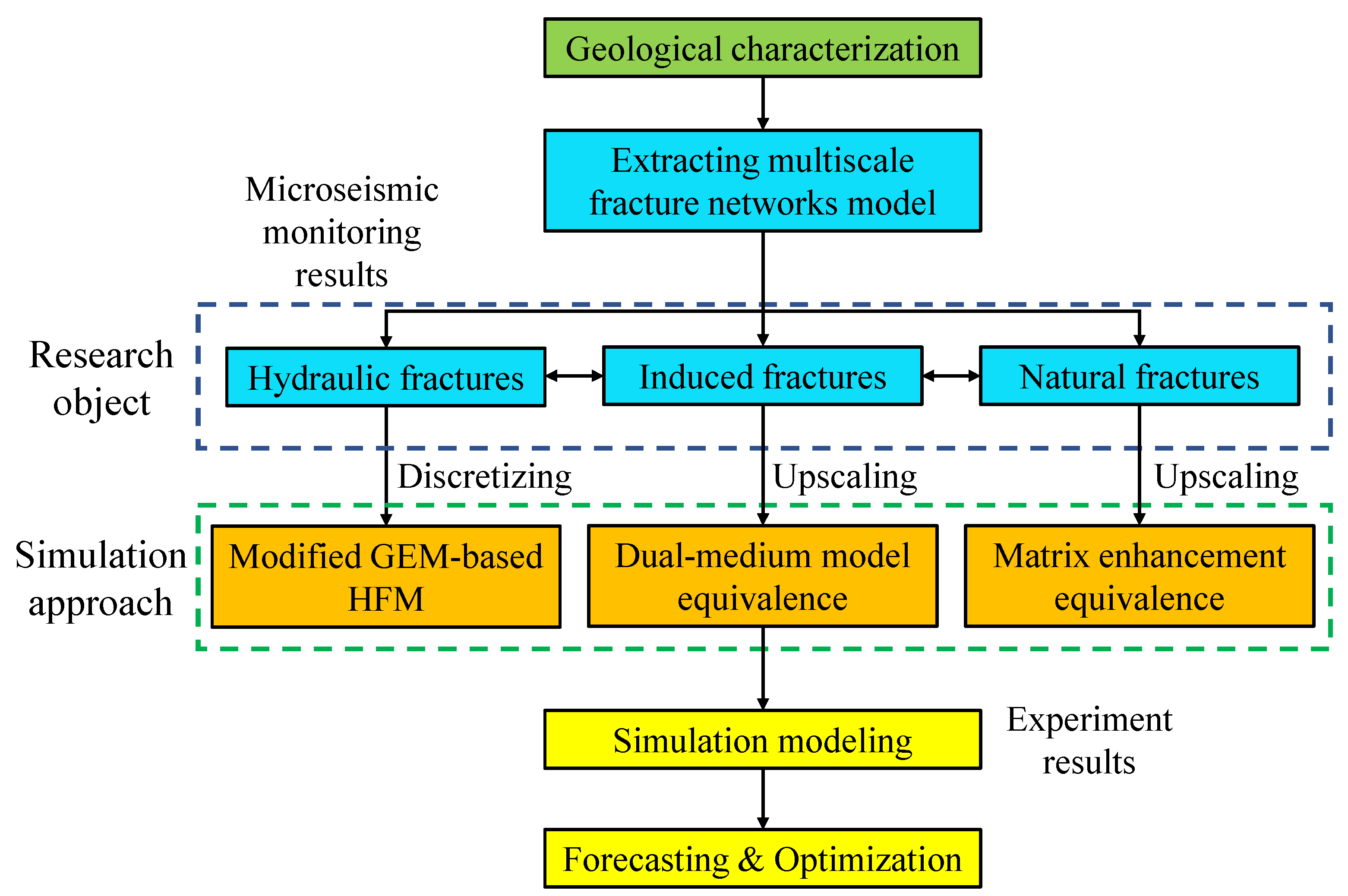
The modeling process of multiscale fractures is mainly divided into 5 steps: (ane) respectively extracting macro-scale fractures, meso-scale fractures, and micro-scale fractures from known information according to the geological characterization of reservoir; (2) macro-scale fractures are modeling past HFM, which corresponds to a set of embedded structured matrix grids. The key of detached scheme is to solve the NNCs between matrix and fractures; (three) equivalently upscaling meso-scale fractures into fractional simulation grids to construct the dual-medium model, which is to calculate dual-medium properties such as the shape factor of fracture grids, the fracture porosity, and the fracture permeability, etc.; (4) equaling backdrop of micro-fractures to fractional matrix grids to grade a single-medium equivalent model; (5) combining the three models to obtain a coupled multiscale fracture networks model.

Due to the simultaneous beingness of embedded detached fractures, dual-medium equivalent fractures, and matrix equivalent fractures, the multi-calibration fracture networks model essentially is a triple-porosity triple-permeability hybrid model containing the discrete fractures, the equivalent fractures, and enhanced matrix. The relationship between the research object (hydraulic fractures, induced fractures, and natural fractures) and the simulation approach is illustrated in an integrated workflow as Figure 5.

three. Model Validation and Analysis

iii.ane. Simulation for Embedded Macro-Fractures

The accuracy of proposed three-dimensional embedded ellipsoidal macro-fracture model is compared with a commercial advanced reservoir-simulation software named tNavigator^® developed by a group named rock catamenia dynamics (RFD), which has become the manufacture standard. The induced fractures and natural fractures are removed in this comparing. The purpose of the showtime example is to verify whether the proposed method can generate capricious-placed fractures in different layers to achieve 3D reservoir simulation. The fractures are vertical in this example considering it is relatively difficult for commercial software to narrate the fractures with capricious dip angles. A fractured inclined-well modeled by proposed method and the 3D reservoir model with fracture elements and the inclined wellbore is shown in Figure vi. The reservoir dimensions are 200 × 200 × twenty m and have two layers. The unlike filigree divisions, such as 20 × 20 × two, 50 × 50 × 2, and 100 × 100 × 2, are used to exam the mesh sensitivity of proposed model. Modeling parameters of reservoir and fluid are shown in Table 1. There are 4 fractures, of which No. 1 and No. three are in the tiptop layer, and No. 2 and No. 4 are in the bottom layer. The fracture parameters in example ane are shown in Table 2. The technology of local filigree refinement (LGR) is used to depict the fractures and the schematic of the grid arrangement with LGR for the commercial simulator tNavigator^® is illustrated every bit Figure vii. The fractured inclined-well is producing at a constant BHP of ten MPa and the simulation fourth dimension for production is 1000 days. The comparing of pressure profiles for different layers betwixt tNavigator^® and our model on the 1000th day is illustrated in Effigy viii and Effigy ix, and the computational results of the 2 models are very similar. Figure 10 shows the difference of the gas production rate of iii simulators (tNavigator^®, original EDFM, and mimetic Precious stone-based HFM) simulating over one thousand days, in which the effect of mesh sensitivity is tested in this comparing between the original model and modified model. The comparison of grid number and average relative errors are shown in Table 3. The result of simulators nether this benchmark proves that the modified model has higher precision and higher robustness than previous EDFMs that prefer a linear steady assumption. The HFM based on mimetic Jewel achieves an accurate calculate of matrix–fracture mass transfer. Consequently, the mesh convergence and accuracy of proposed method in this newspaper are validated when nosotros accept the solution of tNavigator^® as the verbal solution.

In the prior example, the arbitrary-placed fractures in dissimilar layers are modeled by proposed arroyo, and the results are proved to be accurate by comparison with LGR that is represented past a commercial simulator tNavigator^®. The second numerical instance is supplemented to discuss the availability of the characterization model of inclined elliptic fractures. Figure eleven shows the 3D view and overhead view of the reservoir with a three-phase fractured horizontal well, in which it is obvious that some of the fractures are inclined and arbitrarily distributed. The reservoir size is 1000 × 500 × 40 grand and has 4 layers. The modeling parameters of reservoir and fluid are the same as in Table 1. In that location are seven fractures with different azimuth angles, dip angles, lengths, heights, and the reference centre point coordinates of fractures in this example are shown in Table 4. Fractures No. 1, No. 2, No. 3, No. four, and No. five are completely penetrating the 2nd layer and 3rd layer, and partly penetrating the 1st layer and quaternary layer in varying degrees. By dissimilarity, the fracture No. 6 and No. 7 are not penetrating the top layer and the bottom layer because of the cocky-height and inclination degree. The abiding BHP of 10 MPa. The production time is yard days, and the comparing of pressure level profiles for different layers on the 1000th day is shown in Figure 12. Information technology can be seen from this instance that the proposed model can be adaptive to arbitrary inclined fracture with an elliptic shape. Compared with previous EDFMs, this is an innovative characterization method for ellipsoidal-shaped fractures in 3D-reservoir. Compared with the simulator tNavigator^®, the presented approach can handle non only arbitrary-placed fractures but also characterize the fractures with arbitrary dip angles.

iii.two. Simulation for Multi-Calibration CFNs

A staged-fractured horizontal well with a set of multi-calibration CFNs is designed past proposed hybrid model as shown in Effigy xiii. The accurateness and stability of proposed model are compared and verified by commercial simulator tNavigator^®. The reservoir dimensions are 800 × 400 × ten yard and only have one layer. The modeling parameters of the reservoir and fluid are the same as in Table one. To saving the computing cost, all of the fractures are completely penetrating the reservoir and without any arbitrary dip angles. The fracture parameters are shown in Tabular array v and the noticeable differences between unlike scale fractures are length, aperture, and azimuth degree. The multi-scale CFNs are modeled past tNavigator^® and illustrated in Effigy fourteen. In tNavigator^®, the LGR method and DPDK model are used for modeling the hydraulic fractures and induced fractures separately, and the matrix enhancement equivalent approach is adopted for micro-scale fractures. In this instance, the two models keep the same size of grid-block, but the number of fracture elements in tNavigator^® is more than that in our model and this is caused by LGR. The production fourth dimension is 1000 days under a constant BHP of 10 MPa. The comparison of pressure level profiles for multi-scale CFNs in dissimilar periods is shown in Effigy fifteen, the comparing of production dynamics calculated by two simulators over chiliad days is Figure 16, and the comparison of grid number and boilerplate relative errors for 2 simulators is Table 6. The simulation results showed a skillful agreement for pressure profiles, daily product curve, and the boilerplate reservoir pressure curve of two simulators on the one thousand days. The results within a reasonable error range point the loftier accuracy of the proposed hybrid model.

4. Application Instance

In this section, nosotros requite a typical field case that simulates a multi-stage fractured horizontal well to discuss the practicability of proposed model. The studied shale gas well is located in the Sichuan Basin of southwestern Cathay. A sure calibration of natural fractures is developed in this shale formation and all the data come from this expanse. Table 7 shows the modeling parameters of reservoir and fluids, such as rock, fracture, and gas-phase backdrop.The testing results of water saturation testify that the irreducible h2o saturation of shale rock is 28.1~xl.2%, with an average of 34.2%, which is ultra-depression h2o saturation. Additionally, the volume of adsorbed gas in shale core accounts for 27.8% of the total gas volume according to the experiment results.

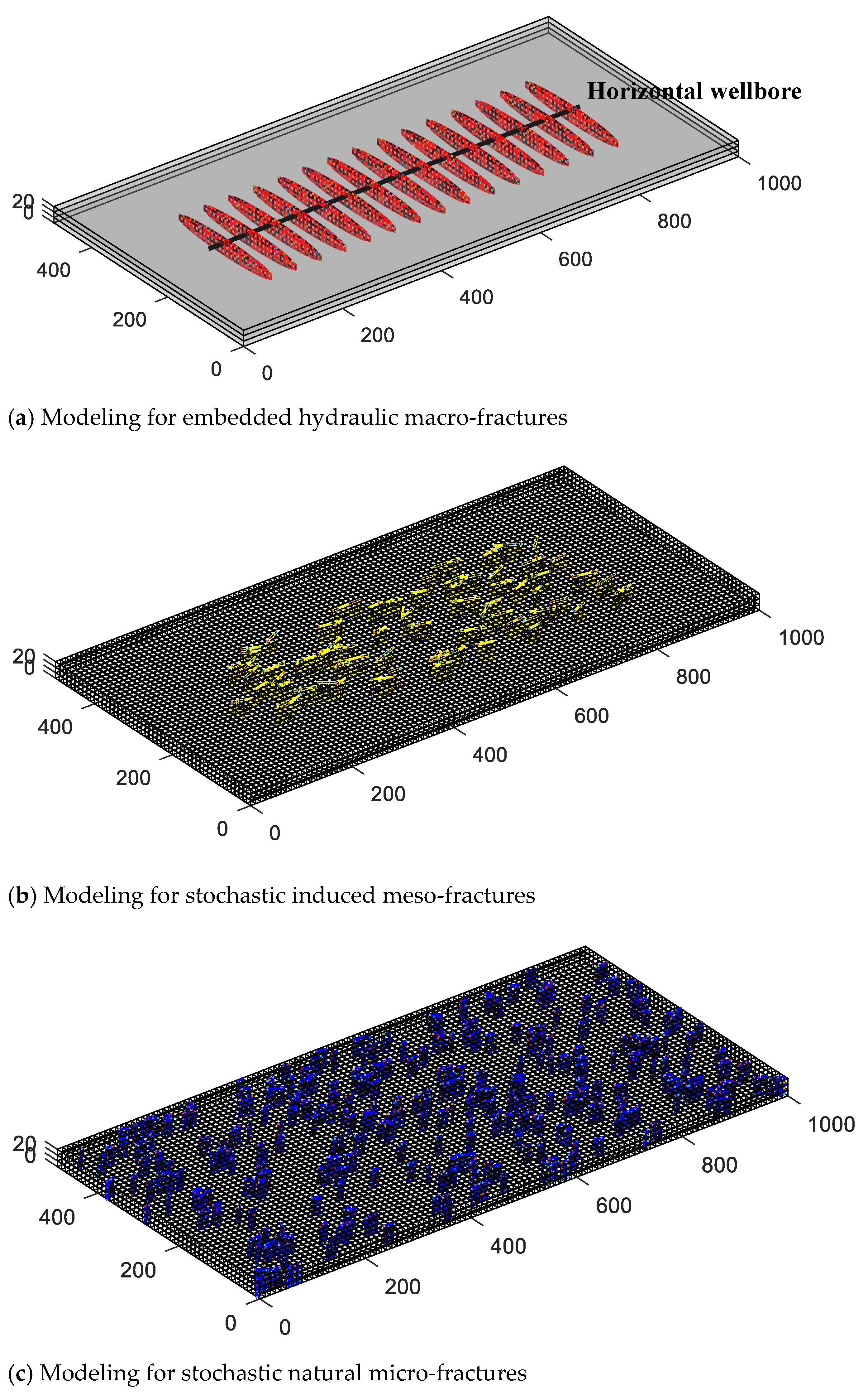
Modeling for multi-calibration fractures is shown in Effigy 17. Firstly, all hydraulic macro-fractures are assumed to be evenly distributed on the horizontal section. The basic model of 3D reservoirs with the embedded macro-fractures and the horizontal wellbore is modeled in Figure 17a. The induced fractures and natural micro-fractures are modeled with the multi-stochastical simulation method according to the bodily situation of shale gas reservoirs. Their respective 3D spatial position coordinates are stochastically generated by the Monte Carlo method [47] and generated in the germination. The difference betwixt them is that the induced fractures just exist in the SRV, while the natural fractures exist in whole reservoirs. The strike of these fractures is determined by multiple-point geostatistics and the tendency of minimum horizontal principal stress is taken as an boilerplate value with a standard deviation is 20°. The full number of meso-scale induced fractures is 70 and its length is adamant by Boolean random simulation with an average value of 35 thousand and the standard divergence of 10 m. Similarly, the total number of natural micro-fractures is 300 and its average value of length is 15m with a standard deviation of five m. The basic model of induced fractures is shown in Effigy 17b. and the natural micro-fractures modeling is shown in Figure 17c. The next step is to find the matrix grid where the meso-calibration and micro-calibration fractures are located and care for them with their respective equivalent methods. Lastly, combining the three models in Effigy 17a, Figure 17b and Effigy 17c to obtain a coupled triple-porosity triple-permeability hybrid model for simulating the multiscale fracture networks. The reservoir pressure distribution map at the different years, in this case, is illustrated in Effigy 18.

Figure nineteen shows the simulation results of germination force per unit area and the gas production rate. At nowadays, this studied fractured horizontal well in Sichuan has been in product for about 6 years. Comparing the production functioning information calculated past proposed model with the field product data, it can be proved that the trend of productivity is highly consistent and the errors were acceptable. The above comparison results explicate that the proposed model has loftier reliability. The development of shale gas reservoirs is dominated by fracture-controlled resources. Therefore, the permeability of each scale fracture is an important evaluation parameter, which straight influences the gas recovery.

5. Conclusions

A hybrid hierarchical fracture modeling framework is proposed in this paper to lucifer the multiscale CFNs and benchmarked with tNavigator^®. The results prove that the proposed model has high precision and loftier robustness. The proposed hybrid model was practical for simulation of a typical well in Sichuan shale, indicating that the proposed method tin provide theoretical guidance for productivity forecasting and optimization. The simulation results show that the multiscale CFNs is an essential consideration affecting the production of gas wells. Generally, the enlightenment for engineering technicians mainly includes two aspects. Firstly, it is very important to establish high-electrical conductivity macro-fractures as preferential channeling, and secondly, it is necessary to increase the area and utilization rate of SRV.

Writer Contributions

X.D. and J.C. (Jun Chen) conceived of the presented idea. X.D. established the model and wrote the manuscript. J.C. (Jianchao Cai) supervised this research and revised the manuscript. 10.D. and Fifty.N. ran the simulation and validated the model. Fifty.C. and R.C. supervised the findings of this work. All authors discussed the results and contributed to the final manuscript. All authors take read and agreed to the published version of the manuscript.

Funding

This inquiry was funded by the National Natural Scientific discipline Foundation of Communist china (Grant Nos. U19B6003, U1762210 and 51774297), National Major Scientific discipline and Technology Projects of Prc (Grant No. 2017ZX05069), and China Petroleum Science and Technology Program (Major Program, Grant No. ZLZX2020-02-04).

Institutional Review Board Statement

Not applicative.

Informed Consent Statement

Non applicative.

Data Availability Statement

Not applicative.

Conflicts of Interest

The authors declare no conflict of interest.

References

1. Wei, W.; Xia, Y. Geometrical, fractal and hydraulic properties of fractured reservoirs: A mini-review. Adv. Geo-Free energy Res. 2017, one, 31–38. [Google Scholar] [CrossRef]
2. Ebrahim, M.; Hassan, D. The fate of fracturing h2o: A field and simulation study. Fuel 2016, 163, 282–294. [Google Scholar]
3. Jia, P.; Cheng, Fifty.-S.; Huang, Due south.-J. Transient beliefs of complex fracture networks. J. Pet. Sci. Eng. 2015, 132, 1–17. [Google Scholar] [CrossRef]
4. Medeiros, F.; Ozkan, E.; Kazemi, H. A semianalytical approach to model pressure transients in heterogeneous reservoirs. SPE Reserv. Eval. Eng. 2010, 13, 341–358. [Google Scholar] [CrossRef]
5. Shakiba, Yard.; Cavalcante, A.; Sepehrnoori, K. Using embedded discrete fracture model (EDFM) in numerical simulation of complex hydraulic fracture networks calibrated by microseismic monitoring data. J. Nat. Gas Sci. Eng. 2018, 55, 495–507. [Google Scholar] [CrossRef]
6. Wu, Y.-H.; Cheng, 50.-S.; Killough, J.E. Integrated label of the fracture network in fractured shale gas reservoirs—Stochastic fracture modeling, simulation and assisted history matching. In Proceedings of the SPE Almanac Technical Briefing and Exhibition, Calgary, AB, Canada, 30 September–two October 2019. [Google Scholar]
7. Lord's day, J.; Niu, G.; Schechter, D. Numerical simulation of stochastically-generated complex fracture networks byutilizing core and microseismic data for hydraulically fractured horizontal wells in unconventional reservoirs—A field example study. In Proceedings of the SPE Eastern Regional Meeting, Canton, OH, USA, 13–15 September 2016. [Google Scholar]
8. Obembe, A.D.; Hossain, M.Due east. A new pseudosteady triple-porosity model for naturally fractured shale gas reservoir. In Proceedings of the SPE Annual Technical Conference and Exhibition, Houston, TX, USA, 28–thirty September 2015. [Google Scholar]
9. Jiang, J.; Younis, R. A multimechanistic multicontinuum model for simulating shale gas reservoir with circuitous fractured arrangement. Fuel 2015, 161, 333–344. [Google Scholar] [CrossRef]
10. Zhang, T.; Li, Z.; Adenutsi, C.D.; Lai, F. A new model for computing permeability of natural fractures in dual-porosity reservoir. Adv. Geo-Free energy Res. 2017, ane, 86–92. [Google Scholar] [CrossRef]
11. Barenblatt, 1000.; Zheltov, I. Bones flow equations for homogeneous fluids in naturally fractured rocks. Doklady Akad. Nauk. 1960, 13, 245–255. [Google Scholar]
12. Warren, J.; Root, P. The beliefs of naturally fractured reservoirs. SPE J. 1963, 3, 245–255. [Google Scholar] [CrossRef]
13. Pruess, M.; Narasimhan, T. On fluid reserves and the production of superheated steam from fractured, vapor-dominated geothermal reservoirs. J. Geophys. Res. 1982, 87, 9329–9339. [Google Scholar] [CrossRef]
14. Pruess, K.; Narasimhan, T. A practical method for modeling fluid and estrus flow in fractured porous media. SPE J. 1985, 25, 14–26. [Google Scholar] [CrossRef]
15. Wu, Y.; Pruess, G. A multiple-porosity method for simulation of naturally fractured petroleum reservoirs. SPE Reserv. Eng. 1988, 3, 327–336. [Google Scholar] [CrossRef]
16. Blaskovich, F.; Cain, G.; Webb, S. A multicomponent isothermal system for efficient reservoir simulation. In Proceedings of the Centre East Oil Technical Conference and Exhibition, Manama, Bahrain, 14–17 March 1983. [Google Scholar]
17. Loma, A.; Thomas, One thousand. A new approach for simulating complex fractured reservoirs. In Proceedings of the Middle East Oil Technical Conference and Exhibition, Manama, Bahrain, 11–fourteen March 1985. [Google Scholar]
18. Moinfar, A.; Narr, W.; Hui, M. Comparison of discrete-fracture and dual-permeability models for multiphase flow in naturally fractured reservoirs. In Proceedings of the SPE Reservoir Simulation Symposium, Woodlands, TX, USA, 21–23 February 2011. [Google Scholar]
19. Noorishad, J.; Mehran, M. An upstream finite element method for solution of transient send equation in fractured porous media. Water Resour. Res. 1982, 18, 588–596. [Google Scholar] [CrossRef]
20. Kim, J.G.; Deo, 1000.D. Finite element discrete-fracture model for multiphase flow in porous media. AIChE J. 2000, 46, 1120–1130. [Google Scholar] [CrossRef]
21. Wang, Y.; Shahvali, 1000. Detached fracture modeling using Centroidal Voronoi grid for simulation of shale gas plays with coupled nonlinear physics. Fuel 2016, 163, 65–73. [Google Scholar] [CrossRef]
22. Lee, S.H.; Lough, M.F.; Jensen, C.Fifty. Hierarchical modeling of flow in naturally fractured formations with multiple length scales. Water Resour. Res. 2001, 37, 443–498. [Google Scholar] [CrossRef]
23. Li, 50.; Lee, Due south.H. Efficient field-calibration simulation of black oil in a naturally fractured reservoir through discrete fracture networks and homogenized media. SPE Reserv. Eval. Eng. 2008, xi, 750–758. [Google Scholar] [CrossRef]
24. Moinfar, A.; Varavei, A.; Sepehrnoori, Thousand. Development of an efficient embedded discrete fracture model for 3D compositional reservoir simulation in fractured reservoirs. SPE J. 2014, xix, 289–303. [Google Scholar] [CrossRef]
25. Snow, D.T. Rock fracture spacings, openings, and porosities closure. J. Soil Mech. Found. Div. 1968, 94, 73–92. [Google Scholar] [CrossRef]
26. Matthäi, S.; Mezentsev, A.; Belayneh, M. Command-volume finite-element two-phase menses experiments with fractured rock represented by unstructured 3D hybrid meshes. In Proceedings of the SPE Reservoir Simulation Symposium, Woodlands, TX, USA, 31 Jan–two February 2005. [Google Scholar]
27. Reichenberger, Five.; Jakobs, H.; Bastian, P. A mixed-dimensional finite book method for ii-phase catamenia in fractured porous media. Adv. H2o Resour. 2006, 29, 1020–1056. [Google Scholar] [CrossRef]
28. Monteagudo, J.; Firoozabadi, A. Control-volume method for numerical simulation of 2-stage immiscible menses in two and three-dimensional discrete fractured media. Adv. H2o Resour. 2004, forty, 7405. [Google Scholar] [CrossRef]
29. Karimi-Fard, G.; Durlofsky, L.J.; Aziz, K. An efficient discrete-fracture model applicative for general-purpose reservoir simulators. SPE J. 2004, ix, 227–260. [Google Scholar] [CrossRef]
30. Hoteit, H.; Firoozabadi, A. An efficient numerical model for incompressible two-stage flow in fractured media. Adv. Water Resour. 2008, 31, 891–905. [Google Scholar] [CrossRef]
31. Cockburn, B.; Karniadakis, K.East.; Shu, C. The development of discontinuous Galerkin methods. In Discontinuous Galerkin Methods; Springer: Berlin/Heidelberg, Deutschland, 2000; pp. iii–l. [Google Scholar]
32. Su, H.; Lei, Z.; Li, J. An effective numerical simulation model of multi-scale fractures in reservoir. Acta Pet. Sin. 2019, 40, 587–593. [Google Scholar]
33. Panfili, P.; Cominelli, A. Simulation of miscible gas injection in a fractured carbonate reservoir using an embedded discrete fracture model. In Proceedings of the Abu Dhabi International Petroleum Exhibition and Conference, Abu Dhabi, United Arab Emirates, 10–13 Nov 2014. [Google Scholar]
34. Fang, Due south.-D.; Cheng, Fifty.-S.; Ayala, L.F. A coupled boundary element and finite element method for the analysis of flow through fractured porous media. J. Pet. Sci. Eng. 2017, 152, 375–390. [Google Scholar] [CrossRef]
35. Cao, R.-Y.; Fang, S.-D.; Jia, P. An efficient embedded detached-fracture model for 2nd anisotropic reservoir simulation. J. Pet. Sci. Eng. 2018, 174, 115–130. [Google Scholar] [CrossRef]
36. Rao, Ten.; Cheng, L.-S.; Cao, R.-Y. An efficient three-dimensional embedded detached fracture model for production simulation of multi-stage fractured horizontal well. Eng. Anal. Spring. Elem. 2019, 106, 473–492. [Google Scholar] [CrossRef]
37. Saidi, A. Simulation of naturally fractured reservoirs. In Proceedings of the SPE Reservoir Simulation Symposium, San Francisco, CA, USA, 15–18 November 1983. [Google Scholar]
38. Tene, 1000.; Bosma, Due south.B.; Al Kobaisi, K.S.; Hajibeygi, H. Projection-based embedded discrete fracture model (pEDFM). Adv. H2o Resour. 2017, 105, 205–221. [Google Scholar] [CrossRef]
39. Nejati, M.; Paluszny, A.; Zimmerman, R.W. A finite chemical element framework for modeling internal frictional contact in three-dimensional fractured media using unstructured tetrahedral meshes. Comput. Methods Appl. Mech. Eng. 2016, 306, 123–150. [Google Scholar] [CrossRef]
40. Zhang, J.; Huang, S.; Cheng, 50.; Xu, W.; Liu, H.; Yang, Y.; Xue, Y. Effect of menstruum machinery with multi-nonlinearity on production of shale gas. J. Nat. Gas Sci. Eng. 2015, 24, 291–301. [Google Scholar] [CrossRef]
41. Yang, Z.; Wang, W.; Dong, M.; Wang, J.; Li, Y.; Gong, H.; Sang, Q. A model of dynamic adsorption–diffusion for modeling gas ship and storage in shale. Fuel 2016, 173, 115–128. [Google Scholar] [CrossRef]
42. Du, 10.; Cheng, L.; Liu, Y.; Rao, 10.; Ma, M.; Cao, R.; Zhou, J. Application of 3D embedded detached fracture model for simulating CO2-EOR and geological storage in fractured reservoirs. IOP Conf. Ser. Globe Environ. Sci. 2020, 467, 012013. [Google Scholar] [CrossRef]
43. Hajibeygi, H.; Karvounis, D.; Jenny, P. A hierarchical fracture model for the iterative multiscale finite book method. J. Comput. Phys. 2011, 230, 8729–8743. [Google Scholar] [CrossRef]
44. Yan, 10.; Huang, Z.; Yao, J.; Li, Y.; Fan, D. An efficient embedded detached fracture model based on mimetic finite difference method. J. Pet. Sci. Eng. 2016, 145, 11–21. [Google Scholar] [CrossRef]
45. Rao, X.; Cheng, L.-Southward.; Cao, R.-Y. A mimetic Light-green element method. Eng. Anal. Spring. Elem. 2019, 99, 206–221. [Google Scholar] [CrossRef]
46. Karimi, F.G.; Firoozabadi, A. Numerical simulation of h2o injection in fractured media using the discrete-fracture model and the Galerkin method. SPE Reserv. Eval. Eng. 2003, six, 117–126. [Google Scholar] [CrossRef]
47. Ritchie, D.; Mildenhall, B.; Goodman, N.D. Decision-making procedural modeling programs with stochastically-ordered sequential Monte Carlo. ACM Trans. Graph. 2015, 34, 105. [Google Scholar] [CrossRef]

Effigy 1. Schematic plot of multiscale fractures distribution after hydraulic fracturing.

Figure 1. Schematic plot of multiscale fractures distribution after hydraulic fracturing.

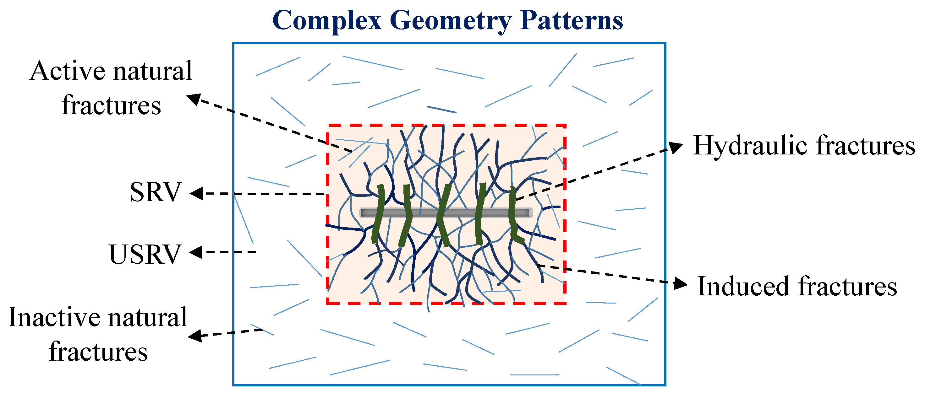
Figure 2. Schematic plot of oblong fracture model (modified from Rao et al. [36]).

Figure 2. Schematic plot of ellipsoidal fracture model (modified from Rao et al. [36]).

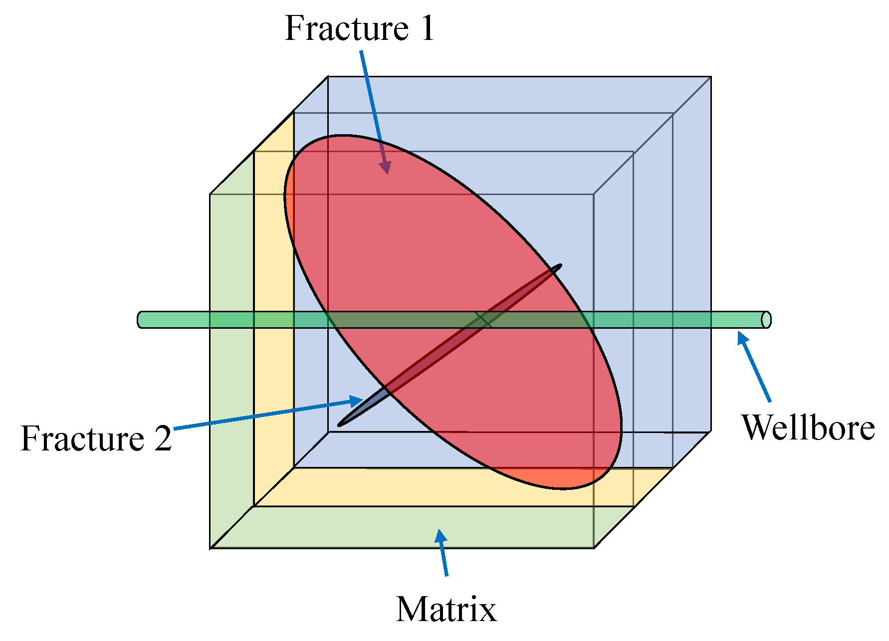
Figure 3. The NNCs of EDFM simulation of macro-fracture.

Effigy 3. The NNCs of EDFM simulation of macro-fracture.

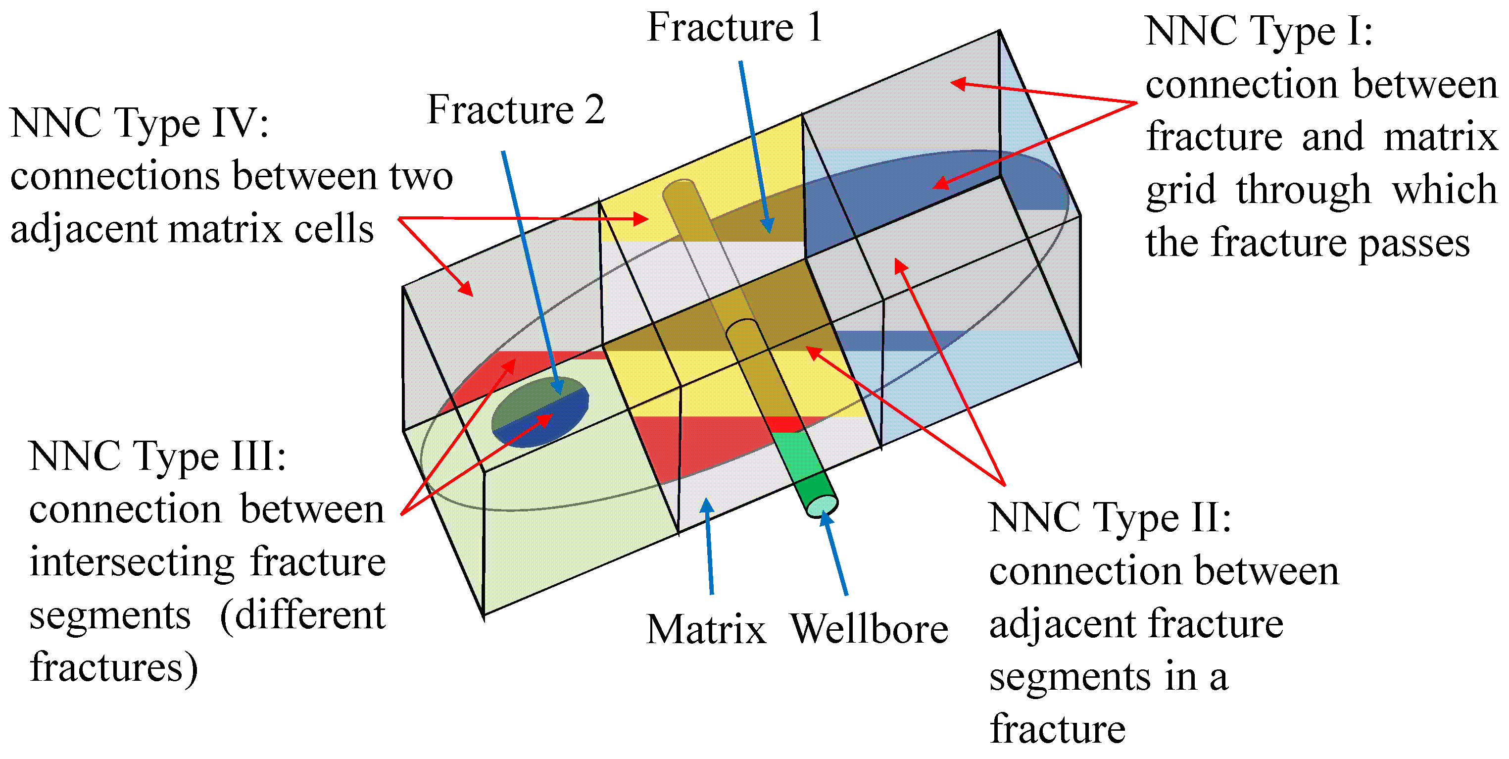
Figure 4. Schematic plot of mimetic Jewel-based HFM in rectangle grid.

Effigy 4. Schematic plot of mimetic Jewel-based HFM in rectangle grid.

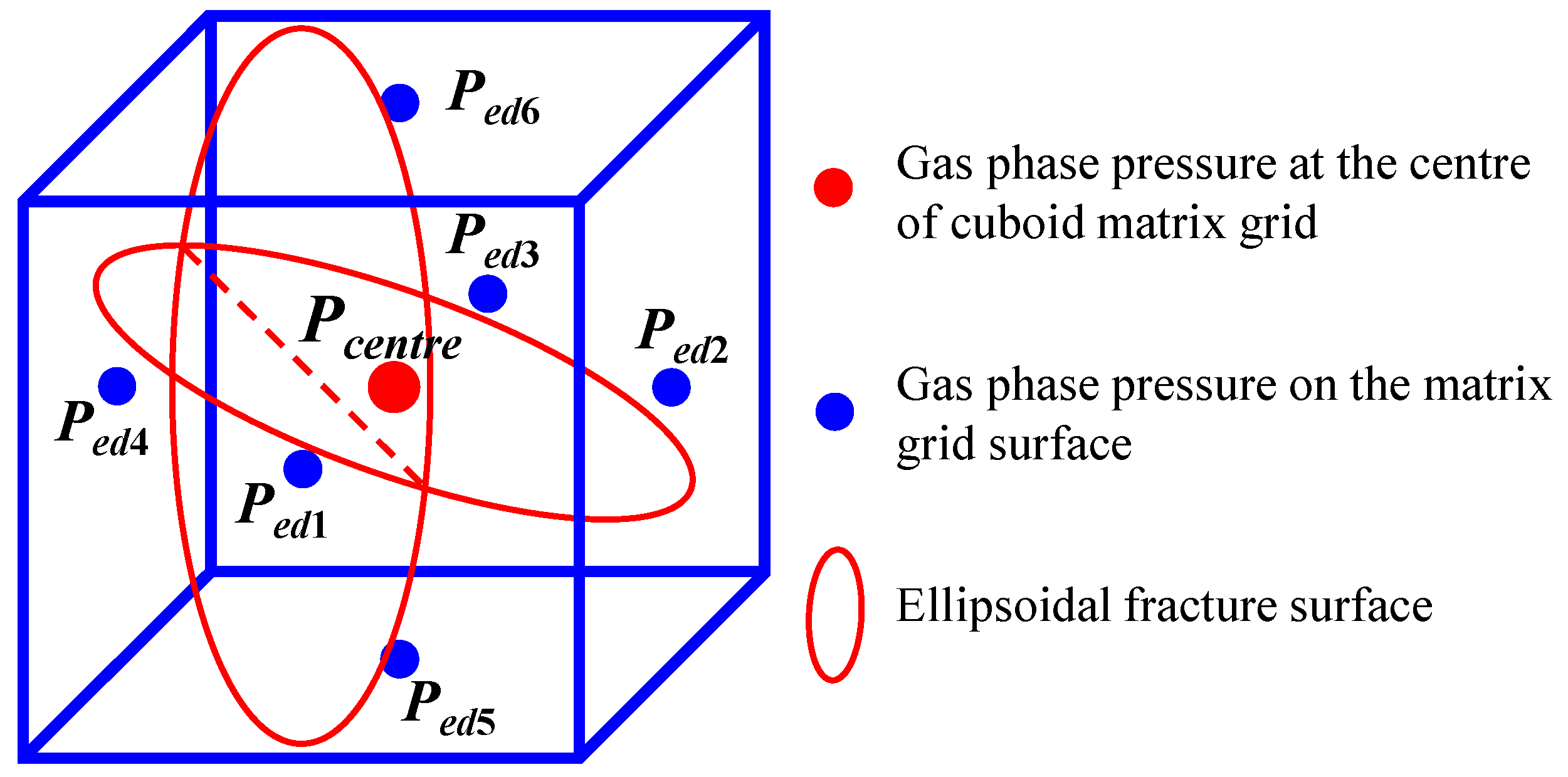
Figure 5. Integrated workflow of multiscale CFNs modeling.

Figure five. Integrated workflow of multiscale CFNs modeling.

Effigy vi. Modeling of 3D reservoir with fracture elements for instance 1.

Effigy 6. Modeling of 3D reservoir with fracture elements for instance 1.

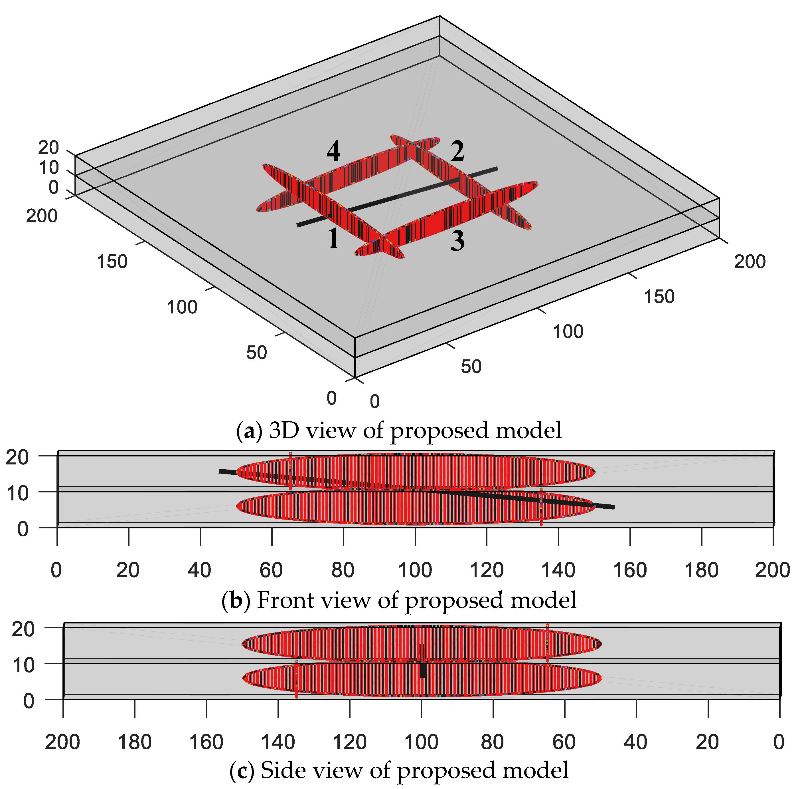
Figure 7. (Left) summit view of the global filigree configuration for macro-fracture. (Right) a view of locally interconnecting fractures and surrounding matrix blocks with permeability distribution in Y-management. The distribution of permeability is also presented in the schematic by using various colors and the permeability distribution in X-direction is the same as that in Y-direction.

Figure seven. (Left) top view of the global grid configuration for macro-fracture. (Right) a view of locally interconnecting fractures and surrounding matrix blocks with permeability distribution in Y-direction. The distribution of permeability is also presented in the schematic by using various colors and the permeability distribution in Ten-direction is the same every bit that in Y-direction.

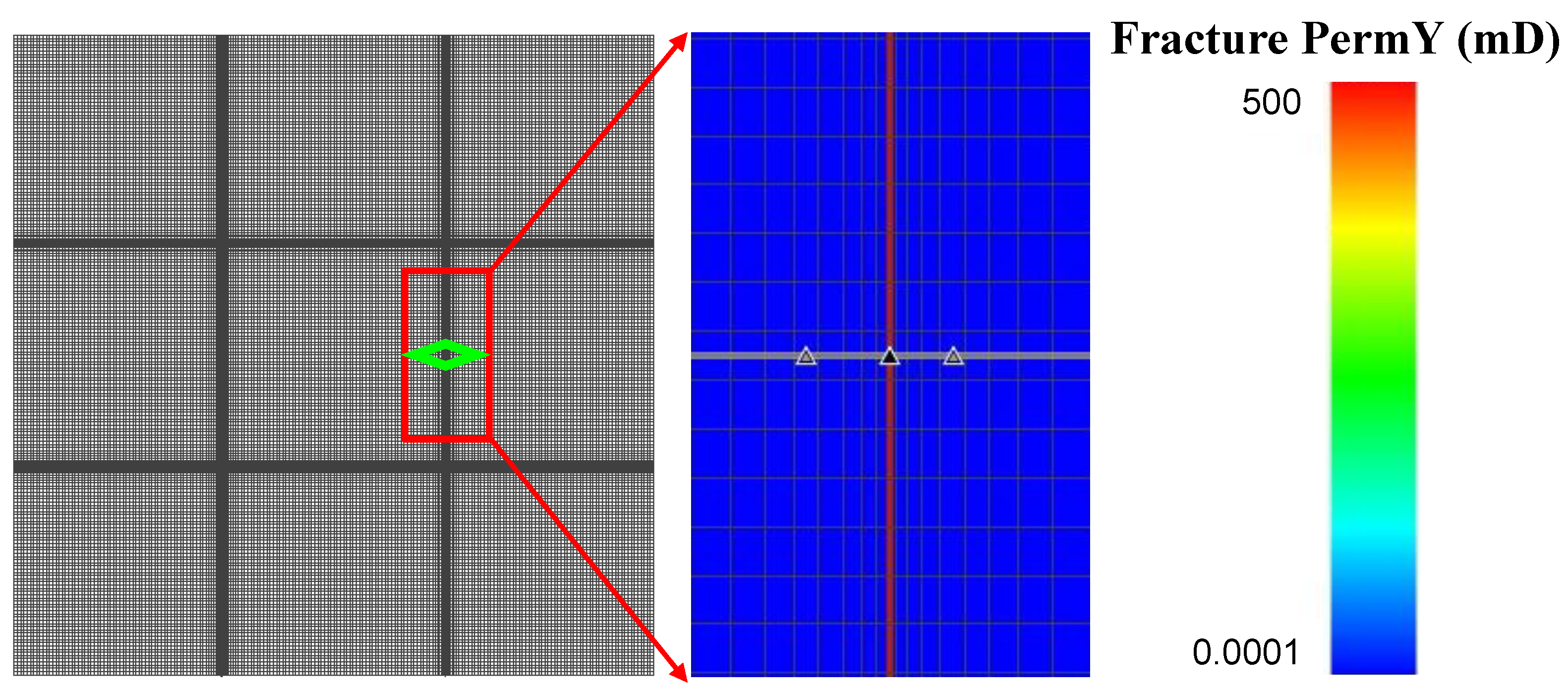
Figure 8. Comparison of pressure level profiles for the top layer on the 1000th twenty-four hour period.

Figure 8. Comparison of pressure profiles for the top layer on the 1000th twenty-four hour period.

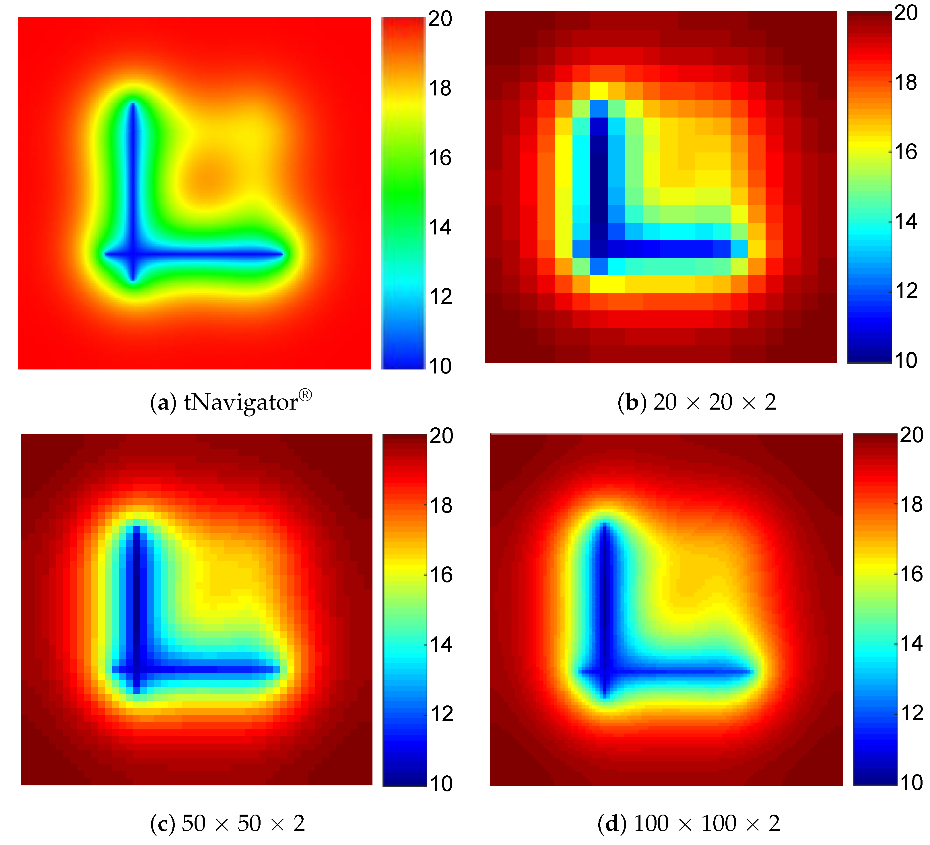
Figure 9. Comparison of pressure profiles for the bottom layer on the 1000th day.

Figure 9. Comparison of pressure profiles for the bottom layer on the 1000th day.

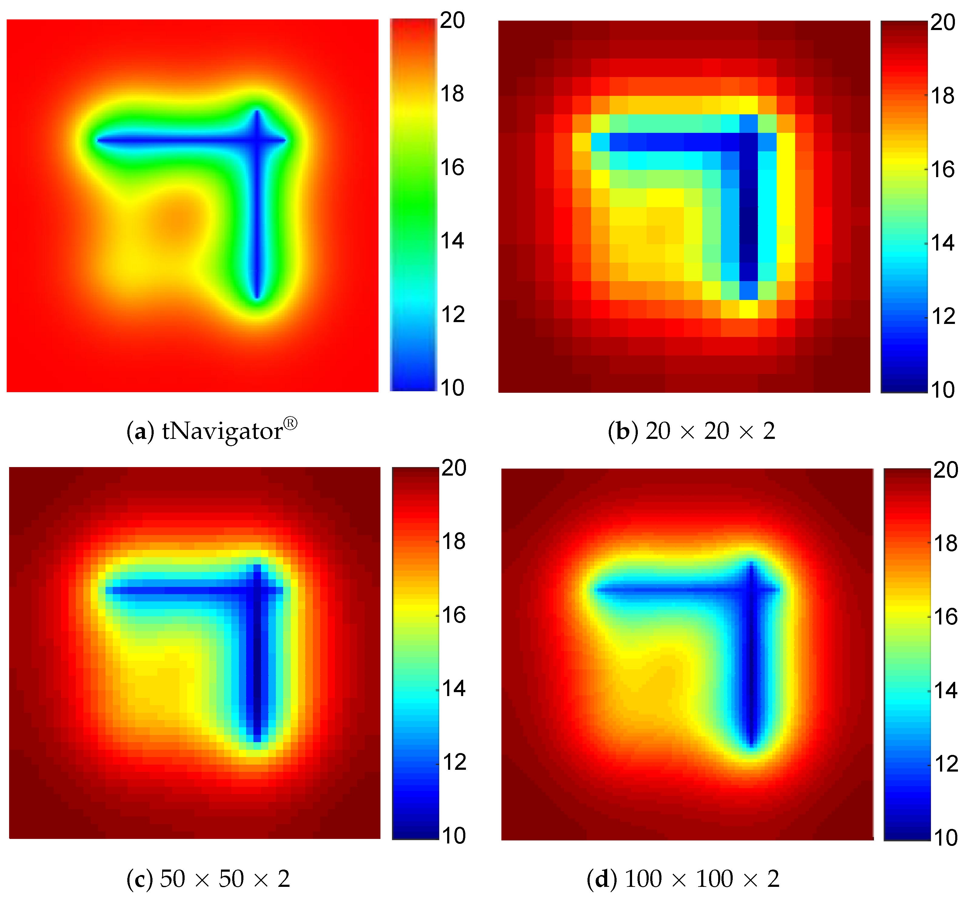
Figure x. Comparing of the gas production rate of various simulators over g days.

Figure ten. Comparison of the gas production rate of various simulators over 1000 days.

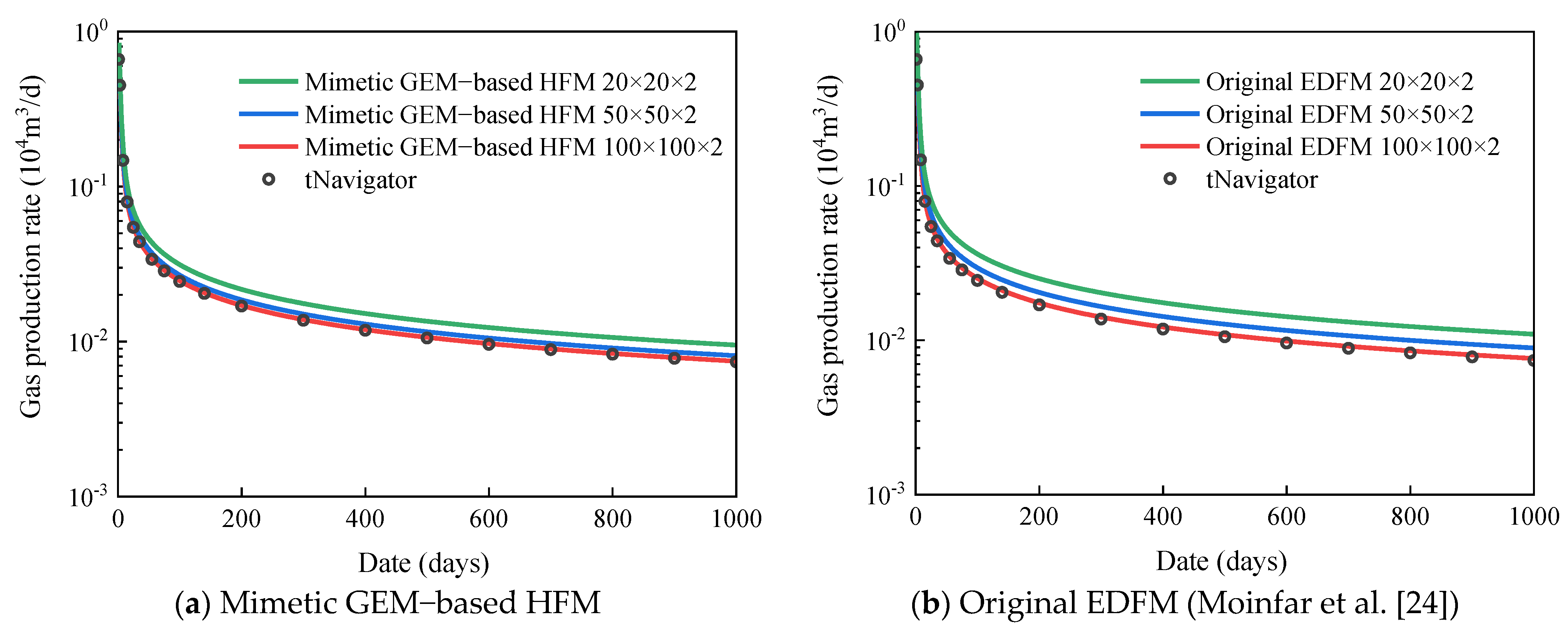
Figure eleven. Modeling of 3D reservoir with fracture elements for example 2.

Figure 11. Modeling of 3D reservoir with fracture elements for example two.

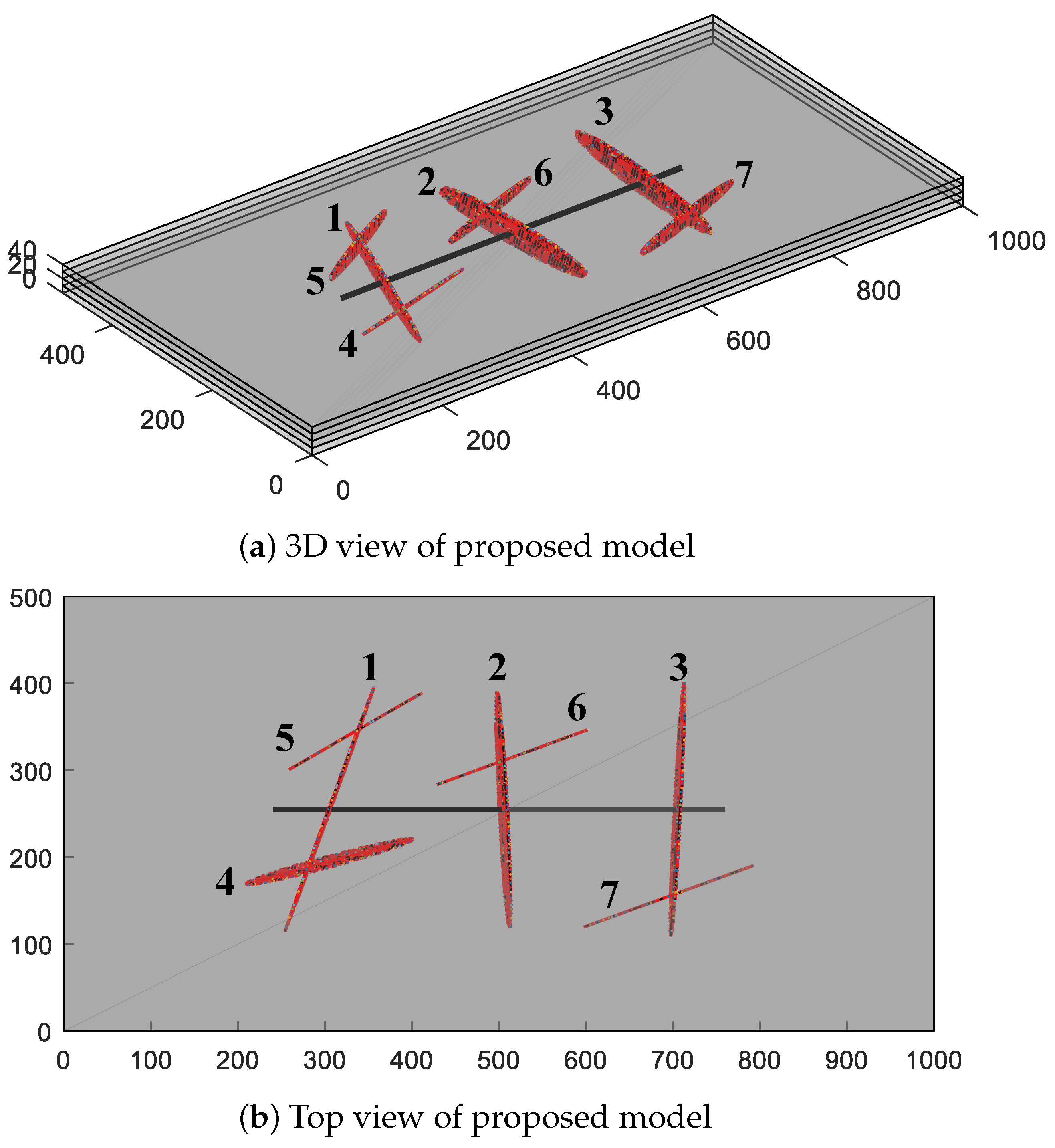
Figure 12. Comparing of pressure profiles for unlike layers on the 1000th twenty-four hours.

Figure 12. Comparing of pressure profiles for different layers on the 1000th day.

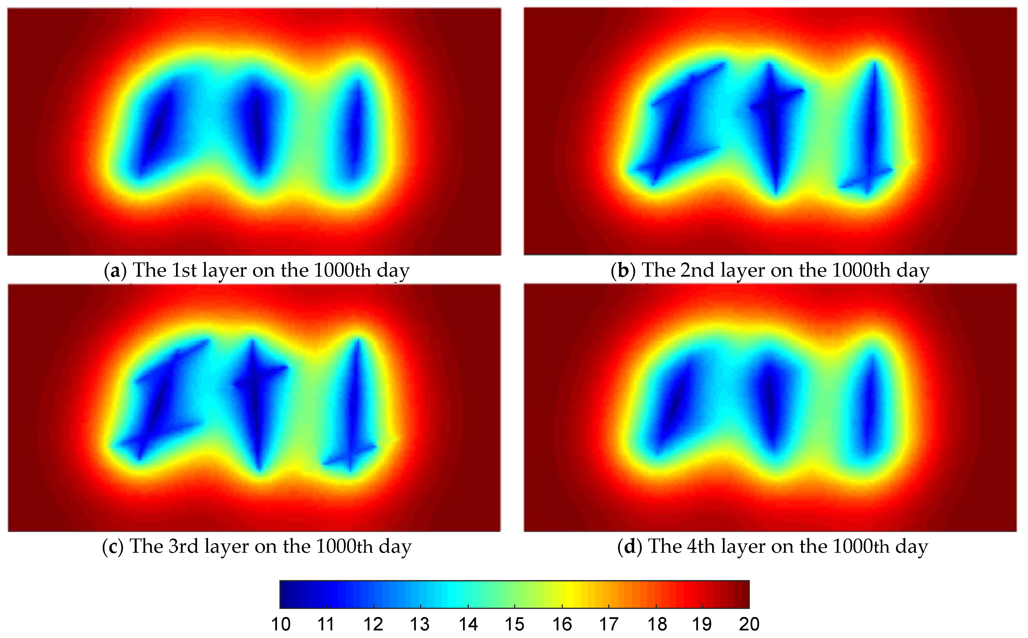
Figure 13. Modeling of the multi-scale CFNs.

Effigy xiii. Modeling of the multi-scale CFNs.

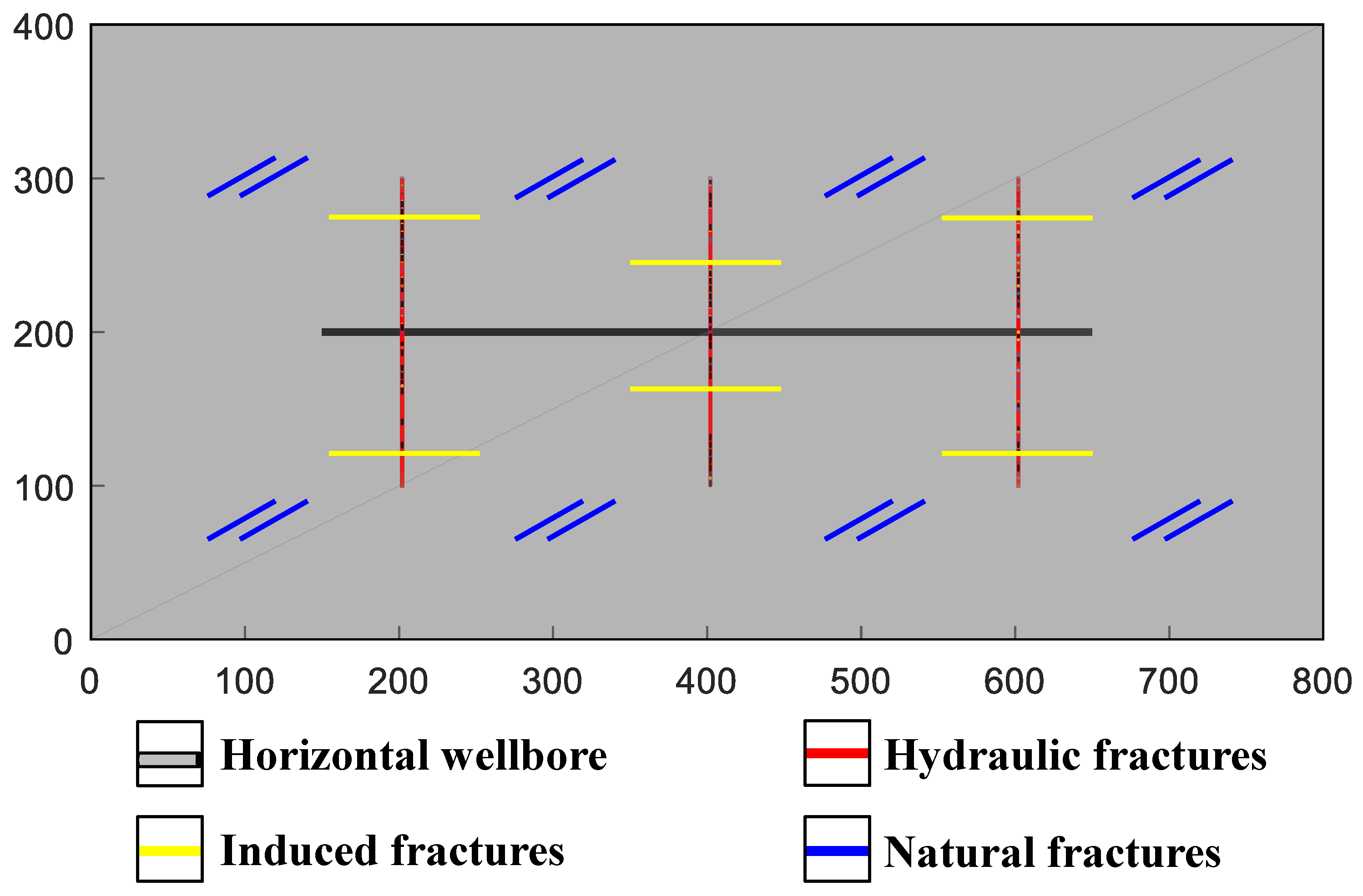
Figure 14. (Left) top view of the global filigree configuration for multi-scale CFNs. (Right) a view of locally interconnecting fractures and surrounding matrix grids with permeability distribution in Y-direction. The distribution of permeability is also presented in the schematic by various colors and the permeability distribution in X-direction is the aforementioned every bit that in Y-direction.

Figure 14. (Left) top view of the global grid configuration for multi-scale CFNs. (Right) a view of locally interconnecting fractures and surrounding matrix grids with permeability distribution in Y-direction. The distribution of permeability is also presented in the schematic by various colors and the permeability distribution in 10-management is the aforementioned every bit that in Y-management.

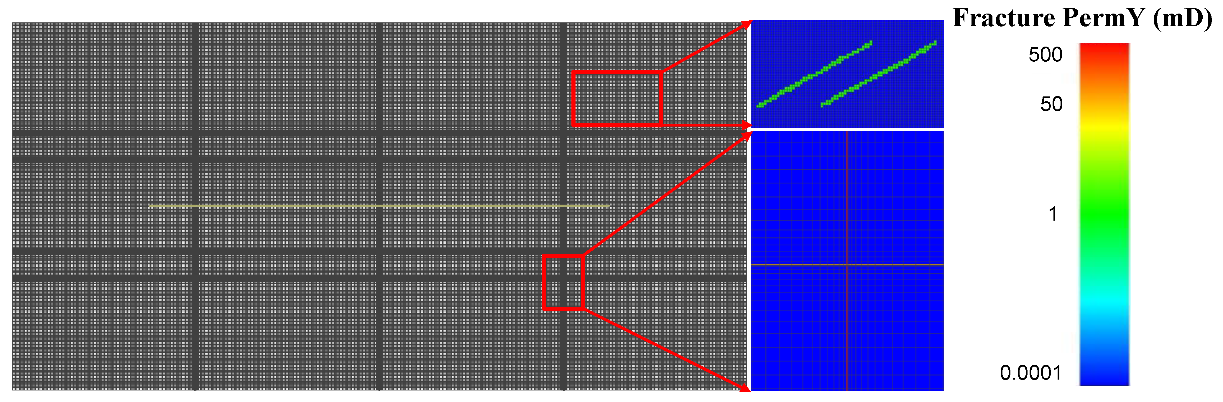
Figure 15. Comparison of pressure profiles for multi-calibration CFNs in different periods.

Figure fifteen. Comparison of pressure profiles for multi-scale CFNs in dissimilar periods.

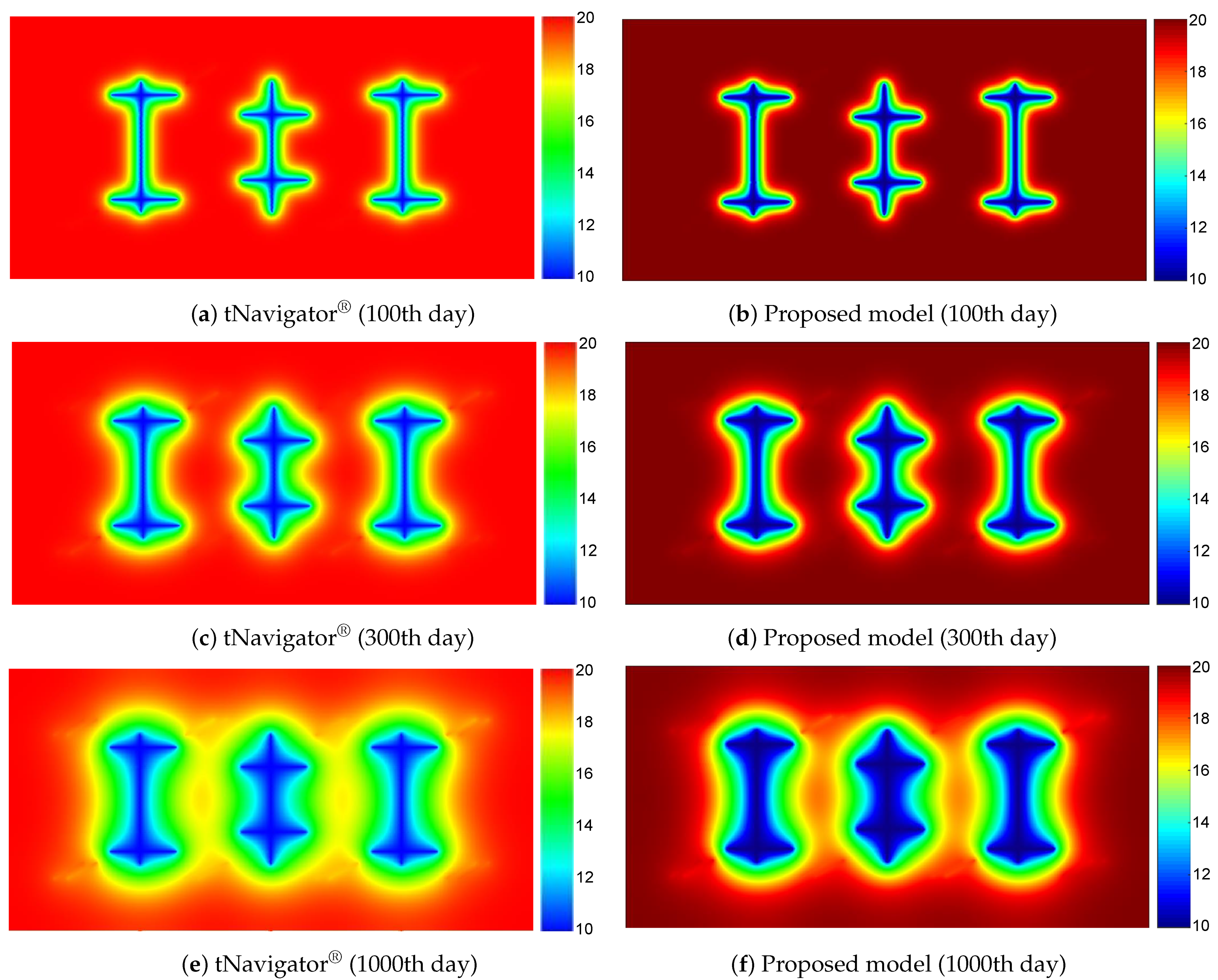
Figure 16. Comparing of production dynamics calculated past two simulators over g days.

Figure sixteen. Comparison of production dynamics calculated by two simulators over m days.

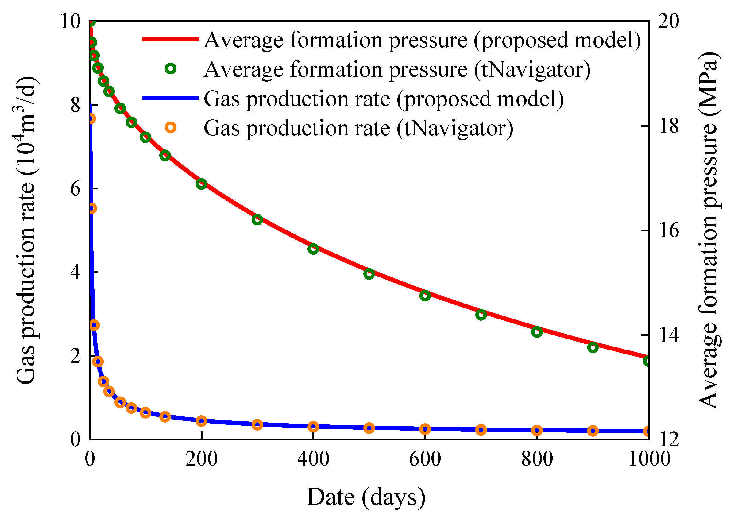
Figure 17. Modeling for multi-scale fractures.

Figure 17. Modeling for multi-scale fractures.

Effigy xviii. Pressure distribution map at the different years in this case.

Figure 18. Pressure distribution map at the dissimilar years in this case.

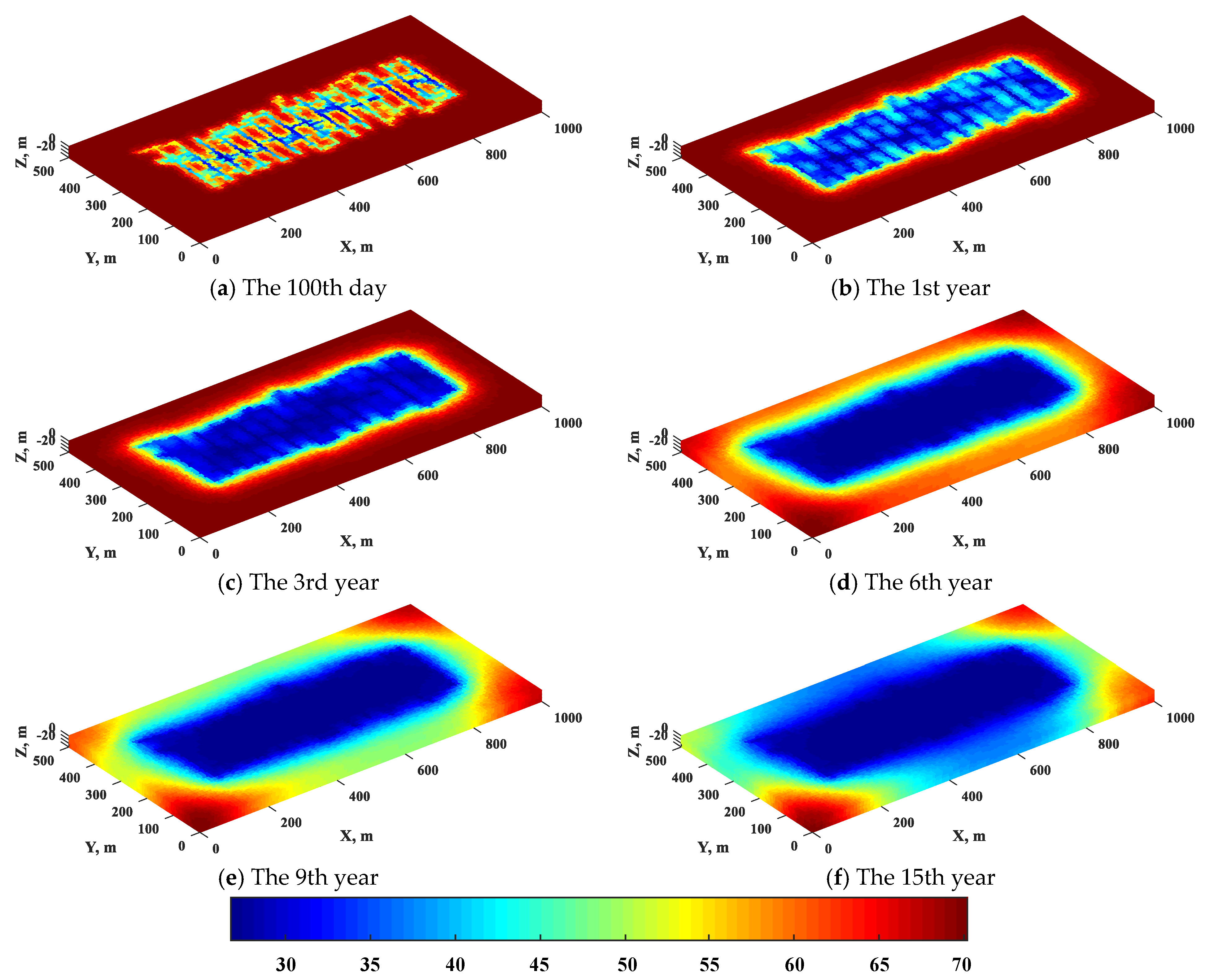
Figure 19. Curves of germination pressure and gas product charge per unit.

Effigy xix. Curves of formation force per unit area and gas production charge per unit.

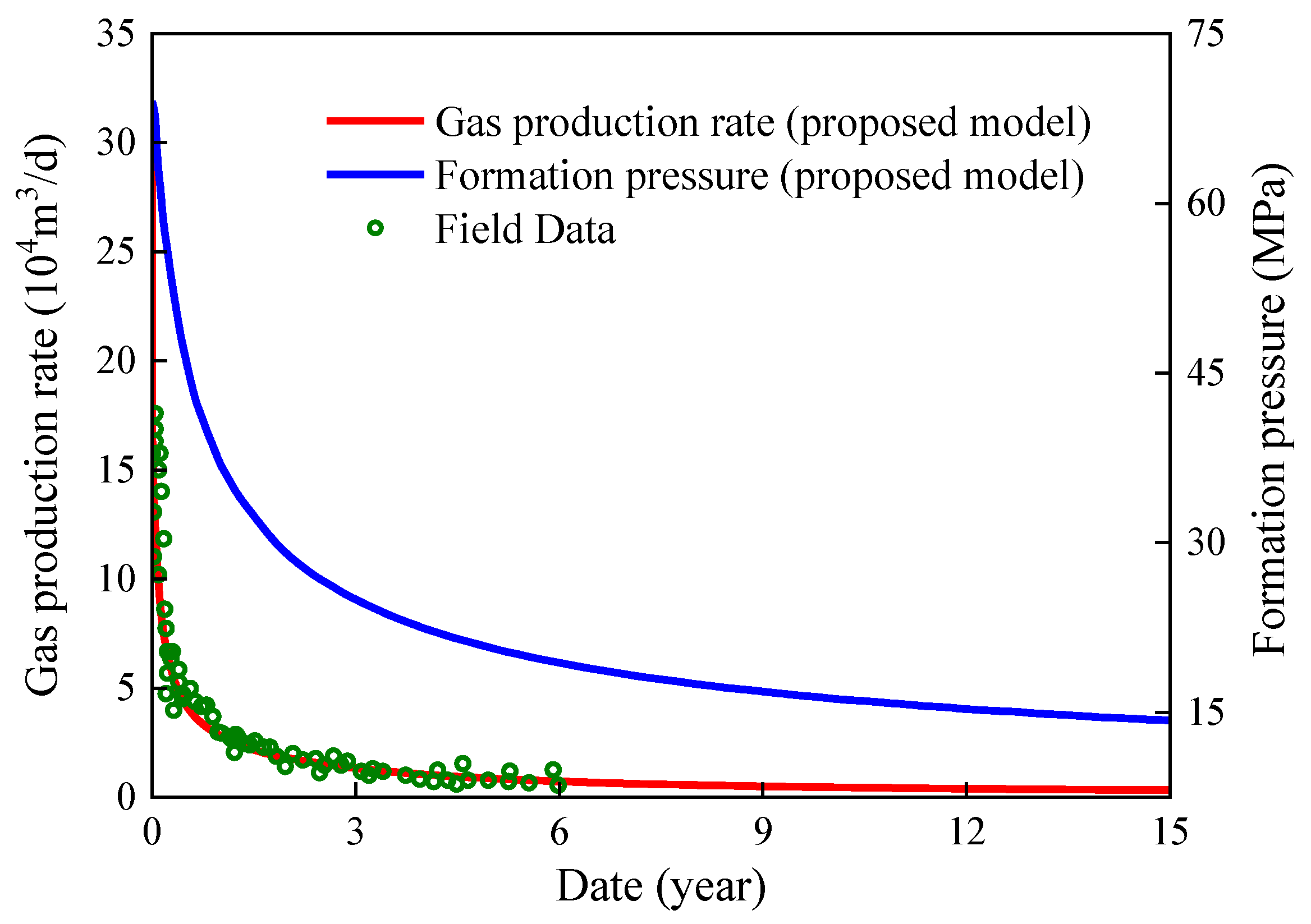
Table 1. Modeling parameters of reservoir and fluid.

Table one. Modeling parameters of reservoir and fluid.

Properties	Value	Properties	Value
Initial reservoir force per unit area, MPa	20	Gas density, fraction	0.72
Gas viscosity, mPa·southward	0.01	Gas Z-factor, fraction	0.viii
Langmuir pressure, MPa	4.8	Langmuir volume, m3/kg	4 × 10−3
Matrix density, kg/m3	2400	Matrix compressibility, MPa−1	one.07 × 10−4
Matrix porosity, fraction	0.1	Matrix permeability, mD	1 × 10−four
Fracture compressibility, MPa−1	one × 10−2	Fracture permeability, physician	500

Tabular array 2. Fracture parameters in example 1.

Table 2. Fracture parameters in example one.

Number	Reference Point Coordinates	Azimuth Bending, °	Fracture Length, m	Fracture Meridian, 1000
i	(65, 100, fifteen)	90	100	x
2	(135, 100, 5)	90	100	10
3	(100, 65, fifteen)	180	100	ten
4	(100, 135, 5)	180	100	x

Table 3. Comparison of grid number and boilerplate relative errors.

Tabular array 3. Comparison of grid number and average relative errors.

Modeling Simulator	Number of Grids	Boilerplate Relative Errors, %
tNavigator® (220 × 220 × two)	96,800	-
Original EDFM (20 × 20 × ii)	800	48.11
Original EDFM (50 × 50 × 2)	5000	21.81
Original EDFM (100 × 100 × 2)	20,000	4.16
Proposed model (20 × 20 × 2)	800	28.24
Proposed model (50 × fifty × 2)	5000	9.59
Proposed model (100 × 100 × two)	20,000	i.08

Table iv. Fracture parameters in example two.

Table 4. Fracture parameters in case ii.

Number	Center Betoken Coordinates	Azimuth Angle, °	Dip Angle, °	Fracture Length, 1000	Fracture Height, m
1	(305, 255, 20)	70	95	300	30
2	(505, 255, 20)	93	70	280	xxx
3	(705, 255, twenty)	87	75	295	30
4	(305, 195, twenty)	15	60	200	25
v	(335, 345, xx)	thirty	xc	180	25
6	(515, 315, 20)	20	88	190	xx
7	(695, 155, 20)	20	xc	210	xv

Table 5. Fracture parameters of multi-scale CFNs.

Table 5. Fracture parameters of multi-calibration CFNs.

Fracture Type	Azimuth Angle, °	Fracture Length, m	Fracture Aperture, mm	Permeability, medico
Hydraulic fracture	ninety	200	1	500
Induced fracture	180	100	0.one	50
Natural fracture	30	50	0.01	one

Table 6. Comparing of grid number and simulation time for two simulators.

Table half dozen. Comparison of filigree number and simulation fourth dimension for two simulators.

Modeling Simulator	Number of Grids	Average Relative Errors, %
tNavigator® (830 × 440 × 1)	365,200	-
Proposed hybrid model (800 × 400 × ane)	320,000	iv.09

Table vii. Modeling parameters of shale reservoir and fluids.

Table 7. Modeling parameters of shale reservoir and fluids.

Properties	Value	Properties	Value
Reservoir volume, m	1000 × 500 × thirty	Filigree number	100 × 50 × 3
Depth, m	2800	Initial reservoir pressure, MPa	69
Horizontal wellbore length, k	805	Well radius, grand	0.18
Skin factor	0.1	Gas density, fraction	0.72
Gas viscosity, mPa·due south	0.01	Gas Z-factor, fraction	0.viii
Langmuir pressure, MPa	4.8	Langmuir volume, m3/kg	4 × 10−3
Matrix density, kg/m3	2400	Matrix compressibility, MPa−i	1.07 × 10−4
Matrix porosity, fraction	0.one	Matrix permeability, mD	6 × ten−4
Fracture number	15	Fracture spacing, m	50
Fracture one-half-length, m	125	Fracture compressibility, MPa−1	1 × x−2
Macro-fracture aperture, mm	i	Macro-fracture permeability, mD	500
Induced-fracture aperture, mm	0.1	Induced-fracture permeability, mD	l
Micro-fracture aperture, mm	0.01	Micro-fracture permeability, doc	one

Publisher's Notation: MDPI stays neutral with regard to jurisdictional claims in published maps and institutional affiliations.

© 2021 by the authors. Licensee MDPI, Basel, Switzerland. This article is an open access commodity distributed nether the terms and conditions of the Creative Eatables Attribution (CC BY) license (https://creativecommons.org/licenses/by/4.0/).

We use cookies on our website to ensure you lot go the best experience.
Read more about our cookies here.

Nosotros take just recently launched a new version of our website.
Help united states to further amend by taking part in this brusque five minute survey here. here.

stammsquished.blogspot.com

Source: https://www.mdpi.com/1996-1073/14/19/6354/htm

Share this post